Fractal Wave Science

1.1 Introduction to Fractal Wave

Equilibrium Fractal Wave was first introduced in Scientific Guide to Price Action and Pattern Trading (2017). The book was written to identify the important market dynamics to predict market movement for trading. The concept of Equilibrium Fractal Wave was born by combining two scientific areas including time series and fractal analysis. In simple term, the Equilibrium Fractal Wave is the combination between Trend and Fractal Wave. The main propositions in the Equilibrium Fractal Wave include:

1. The separate or combined analysis of Trend and Fractal wave is possible.

2. The repeating patterns in Equilibrium Fractal Wave are equivalent to the infinite number of distinctive cycles because the scale of the repeating pattern varies infinitely.

3. Equilibrium Fractal Wave is just a superclass of all the periodic wave patterns we know.

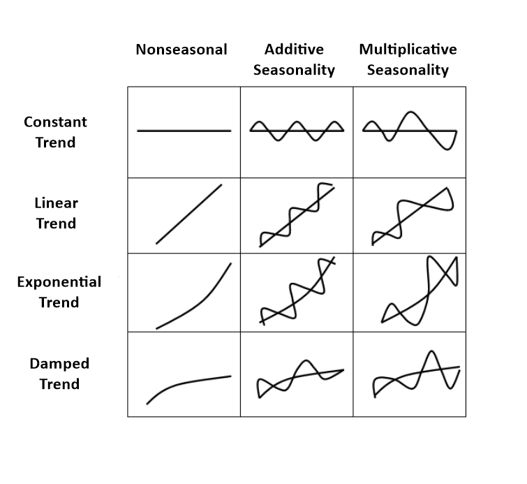
First, let us demonstrate the equilibrium fractal wave for readers. The easiest way to demonstrate the equilibrium fractal wave is through the pattern table presented in Figure 1-1 (Seo, 2017). Many applied researchers in time series and statistics will agree that patterns in the column 1, 2, 3 and 4, from first regularity to fourth regularity, are the mainly extracted features and patterns in their everyday research and operation. It is also agreeable that cyclic wave pattern can co-present with trend together. This concept is the main assumption behind the classic decomposition theory in the time series analysis. In the time series pattern table created by Gardner in 1987 (Figure 1-2) represents this concept clearly. The first row in the pattern table (Figure 1-1) shows the data in which no trend or weak trend exists. The second, third and fourth rows shows the co-existence of trend and waves.

Until now, many forecasting or industrial scientists use such concept to build forecasting models. Likewise, there are many applied software to create the forecasting or prediction model of this kind. Some example forecasting software with such modelling capability includes:

1. Stata (www.stata.com)

2. Eviews (www.eviews.com)

3. IBM SPSS (www.ibm.com/products/spss-statistics)

4. SAS (sas.com)

5. MatLab (www.mathworks.com)

6. And many others

Figure 1-1: Five Regularities and their sub price patterns with inclining trends. Each pattern can be referenced using their row and column number. For example, exponential trend pattern in the third row and first column can be referenced as Pattern (3, 1) in this table.

Figure 1-2: The original Gardner’s table to visualize the characteristics of different time series data (Gardner, 1987, p175). Gardner assumed the three components including randomness, trend and seasonality in this table.

Now the fifth column in Figure 1-1 presents the equilibrium fractal wave. This is extended part from the original Gardner’s table (Figure 1-2). When we list the equilibrium fractal wave in the fifth column, we can see that the pattern table (Figure 1-1) shows a systematic pattern. From left column to right column, we can see that the number of distinctive cycles in the data increases. For example, we can assume the pure trend does not have any periodic cycle. Therefore, number of the distinctive cycle is zero for pure trend series. Under the second and third columns, we can have one to several distinctive cycles depending on if the series follows daily, monthly, and yearly cycles. Under fourth column, we can have many more distinctive cycles outside daily, monthly and yearly cycles but the number of the cycles is finite. Fourier analysis or principal component method can be used to reveal the number of cycles for any series under column 4. From column 1 to column 4, you might be following this systemic pattern pretty well.

However, you might question why equilibrium fractal wave in column 5 possesses such infinite number of distinctive cycles. This is indeed the right question to ask. To understand this, you have to understand the fractal wave first.

A lot of research on fractal analysis was done by B. Mandelbrot (1924-2010). The Book: fractal geometry of nature (Kirkby, 1983) describes the nature of fractal geometries in scientific language. What is the difference between fractal wave and equilibrium fractal wave in this article? Fractal wave views a series as the subject of fractal analysis. Equilibrium Fractal wave views a series as the co-subject of fractal analysis and trend analysis. Hence, equilibrium fractal wave believes co-existence of trend and wave pattern in a single data series. The significance of equilibrium fractal wave is that we can model the trend and fractal wave in two separate steps or in one-step.

Indeed, scientists use the two-step process to model the data in column 2, 3 and 4 in economic and financial research. For example, price series under column 4 can be modelled with trend in the first step. Then the reminding data can be modelled using cycles in the second step. Likewise, for a data series under column 5, we can model a trend part first, then we can model a fractal wave patterns in separate steps. This explains the Proposition 1. This also imposes the fractal analysis under non-stationary condition when the trend component is strong in the data series. In this case, two-step modelling process might be advantageous. When the trend component is less dominating comparing to fractal wave component, the entire price series can be modelled using fractal analysis only. Proposition 1 states that the choice on the modelling process, either one-step or two-steps, is conditional upon the characteristics of the price series.

In the Book: fractal geometry of nature (Kirkby, 1983), the main characteristics of fractal wave is described as the repeating patterns in varying scales. To give you some idea of repeating patterns in varying scales, we can create a synthetic data like that using Weierstrass function. This function is famous for being continuous everywhere but non-differentiable nowhere among the math community. Of course, real world data will never look like this. However, this synthetic data describe what is repeating pattern in varying scale very well for our readers in Figure 1-3. You will see the same patterns everywhere in the data. Small pattern are combined to become the bigger pattern. The resulting bigger patterns look the same like small patterns. As the combing process continues, the size of the pattern can increase infinitely. This is referred to as repeating patterns in varying scale or varying size. This is the core assumption on any fractal analysis.

Now let us walk backwards from this combining process. Let us assume that we can extract those patterns in the same scale from rest and we can put them on the separate paper for each scale. When we separate those patterns in the smallest scale from rest, then the extracted series become the first cycle of our data. This extracted series with one cycle is not different from data or a series in column 2, 3 and 4. Likewise, we can separate the second smallest patterns from rest. This will become second cycle of our data. In this time, the frequency of second cycle will be less comparing to the first cycle because the period of second cycle is greater than first cycle. We can keep continue this separating process to create another cycles. Since we can combine to create the repeating patterns infinitely, we can separate the repeating pattern infinitely too. This describes the proposition 2, the infinite number of distinctive cycle.

Figure 1-3: Weierstrass function to give you a feel for the Fractal-Wave process. Note that this is synthetic Fractal-Wave process only and this function does not represent many of real world cases.

Now the Proposition 2 can lead to the Proposition 3 naturally. As you can see from Figure 1-4, from left to right columns, the number of distinctive cycle increases. Therefore, it is not so hard to say that equilibrium Fractal Wave is a superclass of all the periodic wave patterns we know in column 1, 2, 3 and 4. Figure 1-4 shows this concept clearly to our reader.

Figure 1-4: Visualizing number of distinctive cycle periods for the five regularities. Please note that this is only the conceptual demonstration and the number of cycles for second, third and fourth regularity can vary for different price series.

Finally, in many real world data, we do not possess the highly regular patterns as in a synthetic data like that using Weierstrass function in Figure 1-3. The highly regular repeating patterns are described as the stick self-similarity in In the Book: fractal geometry of nature (Kirkby, 1983). Instead of the strict self-similarity, the real world data will form loose self-similarity shown in Figure 1-5. For the financial price series, we can observe the repeating zigzag patterns made up from so many triangles. The triangles are only similar. However, each triangle in the data will be never identical to the other triangles. This is the typical example of loose self-similarity. This sort of loose self-similarity is much harder to model comparing to the strict self-similarity shown in a synthetic data like that using Weierstrass function (Figure 1-3).

Figure 1-5:  Loose self-similarity in the financial price series.

1.2 Empirical Research on Equilibrium Fractal Wave

As we have described, the concept of equilibrium fractal wave allow us to model the series as the co-subject between trend and fractal wave or as the single subject of fractal wave. The modelling choice will depend on the characteristics of data. Regardless of the modelling choice, Empirical research on equilibrium fractal wave must concern the fractal patterns in data series. Empirical research on equilibrium fractal wave in the price series data is relatively small because mainstream academic research is based on the algorithm utilizing the entire data sets like multiple regression techniques instead of detecting patterns.

One exception is the financial trading community. In the trading community, the repeating patterns or repeating geometry was used as early as 1930s. Some pioneers include R. Schabacker (1932), H.M. Gartley (1935) and R.N. Elliott (1938) in time order. In their books, the various repeating patterns were described for various US stock market data (Figure 1-6, 1-7 and 1-8). Until now, millions of traders are using these patterns in their practical applications for the profiting purpose in forex, future, and stock markets. Figure 1-6, 1-7 and 1-8 shows the commonly used repeating patterns by the financial trader. Having said that these repeating patterns in Figure 1-6, 1-7 and 1-8 were not modelled as the co-subject between trend and fractal wave. Instead, those repeating patterns are only modelled as the subject of fractal wave. Only exception is the trend filtered ZigZag indicator and excessive momentum indicator created recently (Seo, 2018). This is understandable consequence because the idea of equilibrium fractal wave and the two-step modelling process were only introduced in 2017. The modelling technique using trend and fractal wave patterns are only available recently. One very purpose of this article is to inform you that it is possible to model the financial price series as the co-subject between trend and fractal wave in two separate steps.

At the same time, another purpose to create equilibrium fractal wave was to connect the contemporary science to many repeating patterns used by the financial traders. Considering that millions of the financial traders now use the repeating patterns for their every day trading, this is a phenomenal level of activity by the society. Many traders are much happier to use the repeating patterns than the traditional math or technical indicators. Unfortunately, the connection between the repeating patterns and the contemporary science is very poor. It seems no literature is positioning those repeating patterns in the scalable scientific framework. Neither the financial trading community have much idea on what these repeating patterns are and why they are using these patterns. Simply speaking the communication between two communities is blocked. If R.N. Elliott (1938) had a chance to meet B. Mandelbrot (1924-2010), then things may have changed bit. However, they lived in two different time.

The pattern table in Figure 1-1 shows that repeating patterns are merely the extended concept from the conventional mathematical knowledge. We know that it is not so hard to put these five regularities together under the same table. Potential for academic and applied research in equilibrium fractal wave is huge. The main concern is that many techniques used for periodic wave pattern analysis may not work with equilibrium fractal wave because of the infinite number of the distinctive cycle in the data. To the best knowledge, Fourier analysis and many other similar techniques will not handle the infinite number of the distinctive cycle. Therefore, developing new analytical techniques remain as the main challenge for the empirical research in equilibrium fractal wave. In many cases, the algorithm or pattern recognition modelling the price series as the co-subject of trend and fractal wave will improve the prediction accuracy much more.

Figure 1-6: List of triangle and wedge patterns.

Figure 1-7: Ascending Triangle pattern found in USDCAD in H1 chart.

Figure 1-8: Repeating Gartley patterns in Hourly EURUSD Chart Hourly.

1.3 Analogical Reasoning to the Modified Quantum Physics

This section discusses the separate concern from this article. However, this part serves another important purpose for this article. In previous chapter, we have shown that equilibrium fractal wave in column 5 extends the structure of trend and wave in column 2, 3 and 4 of the price pattern table (Figure 1-1). We were able to create the systematic framework for data with zero to infinite number of distinctive cycles. For convenience, we will call the wave and trend structure as equilibrium wave as shown in Figure 1-9. Equilibrium wave is common data structure found in real world. The important characteristic of Equilibrium wave is the finite number of periodic cycles. The cycles in equilibrium wave are periodic and we can measure how long the cycle lasts with our stopwatch. Many social and non-social data can show strong behaviour of equilibrium wave too. The periodic cycles can be modelled well using Fourier analysis and other similar techniques. As we know, Fourier analysis and the quantum physics have a strong connection. Fourier analysis can be used to decompose a typical quantum mechanical wave function. In addition, the trend part of equilibrium wave and particle part of quantum physics can be modelled through many common analysis techniques in the statistics, signal processing, and object tracking field too, for example, Kalman filter or similar techniques. Therefore, it is not so harsh to say that equilibrium wave in column 2, 3 and 4 in Figure 1-1 closely resembles the idea of wave and particle duality of the quantum physics.

To the best knowledge, both data structure is not 100% compatible. However, there is certainly some compatible structure between equilibrium wave and wave-particle duality. For this reason, we could make some analogical reasoning here. As we can extend the classic wave pattern into equilibrium fractal wave pattern (Figure 1-1), we might be able to extend the quantum physics further to deal with the infinite number of distinctive cycles. It is often heard that many quantum physics based algorithms fail to bring the profits or good prediction in the financial trading. The reason might be that the contemporary quantum physics is not dealing with the infinite number of distinctive cycles present in the data. Although this might be just guess for now, the modified quantum physics might work better in the financial trading than the contemporary quantum physics. If they do so, then the modified quantum physics can possibly lead to the potential technological breakthrough in developing better medicine and better spaceship in the future. This is just some research ideas for those working in physics in a hope to provide some alternative solutions to many unsolved problems in this world.

---

EFW Analytics provide the graphic rich and fully visual trading styles. In default trading strategy, you will be looking at the combined signal from Superimposed pattern + EFW Channel or Superimposed pattern + Superimposed Channel. In addition, you can perform many more trading strategies in a reversal and breakout mode. You can also run two different timeframes in one chart to enforce your trading decision. Sound alert, email and push notification are built inside the indicator.

Below is the link to the EFW Analytics:

https://algotrading-investment.com/portfolio-item/equilibrium-fractal-wave-analytics/

https://www.mql5.com/en/market/product/27703

https://www.mql5.com/en/market/product/27702

---

1.4 References

Alexander, C. (2008) Market Risk Analysis, Practical Financial Econometrics (The Wiley Finance Series) (Volume II), Wiley.

Algina, J. & Keselman, H. J. (2000) Cross-Validation Sample Sizes, Applied Psychological Measurement, 24(2), 173-179.

Arlot, S. & Celisse, A. (2010) A survey of cross-validation procedures for model selection, Statistics Surveys, 4(0), 40-79.

Babyak, M. A. (2004) What You See May Not Be What You Get: A Brief, Nontechnical Introduction to Overfitting in Regression-Type Models, Psychosomatic Medicine, 66(3), 411-421.

Brown, L. D. & Rozeff, M. S. (1979) Univariate Time-Series Models of Quarterly Accounting Earnings per Share: A Proposed Model, Journal of Accounting Research, 17(1), 179-189.

Callen, J. L., Kwan, C. C. Y., Yip, P. C. Y. & Yuan, Y. (1996) Neural network forecasting of quarterly accounting earnings, International Journal of Forecasting, 12(4), 475-482.

Carney, S.M. (2010) Harmonic Trading. Profiting from the Natural Order of the Financial Markets (Vol. 1). Pearson Education, Inc.

Cawley, G. C. & Talbot, N. L. C. (2007) Preventing Over-Fitting during Model Selection via Bayesian Regularisation of the Hyper-Parameters, J. Mach. Learn. Res., 8, 841-861.

Chakraborty, K., Mehrotra, K., Mohan, C. K. & Ranka, S. (1992) Forecasting the behavior of multivariate time series using neural networks, Neural Networks, 5(6), 961-970.

Chatfield, C. (1993) Calculating Interval Forecasts, Journal of Business & Economic Statistics, 11(2), 121-135.

Elliott, R. N., Douglas, D. C., Sherwood, M. W., Laidlaw, D. & Sweet, P. (1948) The wave principle (Note that first formal publication date of The Wave Principle was August 31 1938).

Elliott, R. N. (1982) Nature’s Law: The Secret of the Universe, Institute for Economic & Financial Research.

Ernst, J. & Bar-Joseph, Z. (2006) STEM: a tool for the analysis of short time series gene expression data, BMC Bioinformatics, 7(1), 191.

Foster, G. (1977) Quarterly Accounting Data: Time-Series Properties and Predictive-Ability Results, The Accounting Review, 52(1), 1-21.

Frost, A. J. & Prechter, R. R. (2005) Elliott wave principle: key to market behavior, Elliott Wave International.

Gann, W. D. (1996) Truth of the stock tape and Wall Street stock selector, Health Research Books.

Gardner, E. S. (JUN.) (1987). Chapter 11: Smoothing methods for short-term planning and control, The Handbook of forecasting – A Manager’s Guide, Second Edition, Makridakis, S. and Steven C. Wheelright (Edit.), John Wiley & Sons, USA, 174 -175.

Gartley, H. M. (1935) Profits in the stock market, Health Research Books.

Goldberger, A. L., Amaral, L. A. N., Glass, L., Hausdorff, J. M., Ivanov, P. C., Mark, R. G., Mietus, J. E., Moody, G. B., Peng, C.-K. & Stanley, H. E. (2000) PhysioBank, PhysioToolkit, and PhysioNet, Components of a New Research Resource for Complex Physiologic Signals, 101(23), e215-e220.

Goldberger, A. L. & Rigney, D. R. (1991) Nonlinear Dynamics at the Bedside in Glass, L., Hunter, P. and McCulloch, A., eds., Theory of Heart: Biomechanics, Biophysics, and Nonlinear Dynamics of Cardiac Function, New York, NY: Springer New York, 583-605.

Hill, T., O’Connor, M. & Remus, W. (1996) Neural Network Models for Time Series Forecasts, Management Science, 42(7), 1082-1092.

Hsieh, W. W. (2004) Nonlinear multivariate and time series analysis by neural network methods, Reviews of Geophysics, 42(1), RG1003.

Kaastra, I. & Boyd, M. (1996) Designing a neural network for forecasting financial and economic time series, Neurocomputing, 10(3), 215-236.

Kang, S. Y. (1992) An investigation of the use of feedforward neural networks for forecasting, unpublished thesis Kent State University.

Kirkby, M. J. (1983) The fractal geometry of nature. Benoit B. Mandelbrot. W. H. Freeman and co., San Francisco, 1982. No. of pages: 460. Price: £22.75 (hardback), Earth Surface Processes and Landforms, 8(4), 406-406.

Knofczynski, G. T. & Mundfrom, D. (2008) Sample Sizes When Using Multiple Linear Regression for Prediction, Educational and Psychological Measurement, 68(3), 431-442.

Krogh, A. & Hertz, J. A. (1992) A Simple Weight Decay Can Improve Generalization, In Advances in Neural Information Processing Systems 4, 950-957.

Lawrence, S., Giles, C. L. & Tsoi, A. C. (1997) Lessons in neural network training: overfitting may be harder than expected, in Proceedings of the fourteenth national conference on artificial intelligence and ninth conference on Innovative applications of artificial intelligence, Providence, Rhode Island, 1867490: AAAI Press, 540-545.

Liang, Z., Feng, Z. & Guangxiang, X. (2012) Comparison of Fractal Dimension Calculation Methods for Channel Bed Profiles, Procedia Engineering, 28, 252-257.

Liu, Y., Starzyk, J. A. & Zhu, Z. (2008) Optimized approximation algorithm in neural networks without overfitting, IEEE Trans Neural Netw, 19(6), 983-95.

Lodwich, A., Rangoni, Y. & Breuel, T. (2009) Evaluation of robustness and performance of Early Stopping Rules with Multi Layer Perceptrons, translated by  1877-1884.

Luo, X., Patton, A. D. & Singh, C. (2000) Real power transfer capability calculations using multi-layer feed-forward neural networks, Power Systems, IEEE Transactions on, 15(2), 903-908.

Mackey, D. (1991) Bayesian Methods for Adaptive Models, PhD Thesis, California Institute of Technology.

Pesavento, L. & Shapiro, S. (1997) Fibonacci Ratios with Pattern Recognition.

Pesavento, L. & Jouflas, L. (2010) Trade what you see: how to profit from pattern recognition, John Wiley & Sons.

Prechelt, L. (2012) Early Stopping — But When? in Montavon, G., Orr, G. and Müller, K.-R., eds., Neural Networks: Tricks of the Trade, Springer Berlin Heidelberg, 53-67.

Qi, M. & Zhang, G. P. (2001) An investigation of model selection criteria for neural network time series forecasting, European Journal of Operational Research, 132(3), 666-680.

Rao, C. R. & Wu, Y. (2005) Linear model selection by cross-validation, Journal of Statistical Planning and Inference, 128(1), 231-240.

Sabo, D. & Xiao-Hua, Y. (2008) A new pruning algorithm for neural network dimension analysis, translated by  3313-3318.

Schabacker, R. (1932) Technical Analysis and Stock Market Profits, Harriman House Limited.

Schittenkopf, C., Deco, G. & Brauer, W. (1997) Two Strategies to Avoid Overfitting in Feedforward Networks, Neural Networks, 10(3), 505-516.

Schöneburg, E. (1990) Stock price prediction using neural networks: A project report, Neurocomputing, 2(1), 17-27.

Seo, Y. H. (2017) Scientific Guide to Price Action and Pattern Trading, Algotrading-Investment.com, Retrieved from www.amazon.com/dp/B073T3ZMBR

Srinivasan, D., Liew, A. C. & Chang, C. S. (1994) A neural network short-term load forecaster, Electric Power Systems Research, 28(3), 227-234.

Tashman, L. J. (2000) Out-of-sample tests of forecasting accuracy: an analysis and review, International Journal of Forecasting, 16(4), 437-450.

Tkacz, G. (2001) Neural network forecasting of Canadian GDP growth, International Journal of Forecasting, 17(1), 57-69.

Ubeyli, E. D. & Guler, I. (2005) Improving medical diagnostic accuracy of ultrasound Doppler signals by combining neural network models, Comput Biol Med, 35(6), 533-54.

Wang, W., Gelder, P. H. A. J. M. V. & Vrijling, J. K. (2005) Some issues about the generalization of neural networks for time series prediction, in Proceedings of the 15th international conference on Artificial neural networks: formal models and their applications – Volume Part II, Warsaw, Poland, 1986178: Springer-Verlag, 559-564.

Wong, W. K., Xia, M. & Chu, W. C. (2010) Adaptive neural network model for time-series forecasting, European Journal of Operational Research, 207(2), 807-816.

Zaiyong Tang, de Almeida, C. & Fishwick, P. A. (1991) Time series forecasting using neural networks vs. Box- Jenkins methodology, SIMULATION, 57(5), 303-310.

Zhai, Y., Hsu, A. & Halgamuge, S. K. (2007) Combining News and Technical Indicators in Daily Stock Price Trends Prediction, in Proceedings of the 4th international symposium on Neural Networks: Advances in Neural Networks, Part III, Nanjing, China, 1419174: Springer-Verlag, 1087-1096.

Zhang, G., Eddy Patuwo, B. & Y. Hu, M. (1998) Forecasting with artificial neural networks:: The state of the art, International Journal of Forecasting, 14(1), 35-62.

Zhang, G. P. (2003) Time series forecasting using a hybrid ARIMA and neural network model, Neurocomputing, 50(0), 159-175.

Zhang, G. P. & Kline, D. M. (2007) Quarterly Time-Series Forecasting With Neural Networks, Neural Networks, IEEE Transactions on, 18(6), 1800-1814.

Related Products