Equilibrium Fractal-Wave Process (Trend and Fractal Wave)
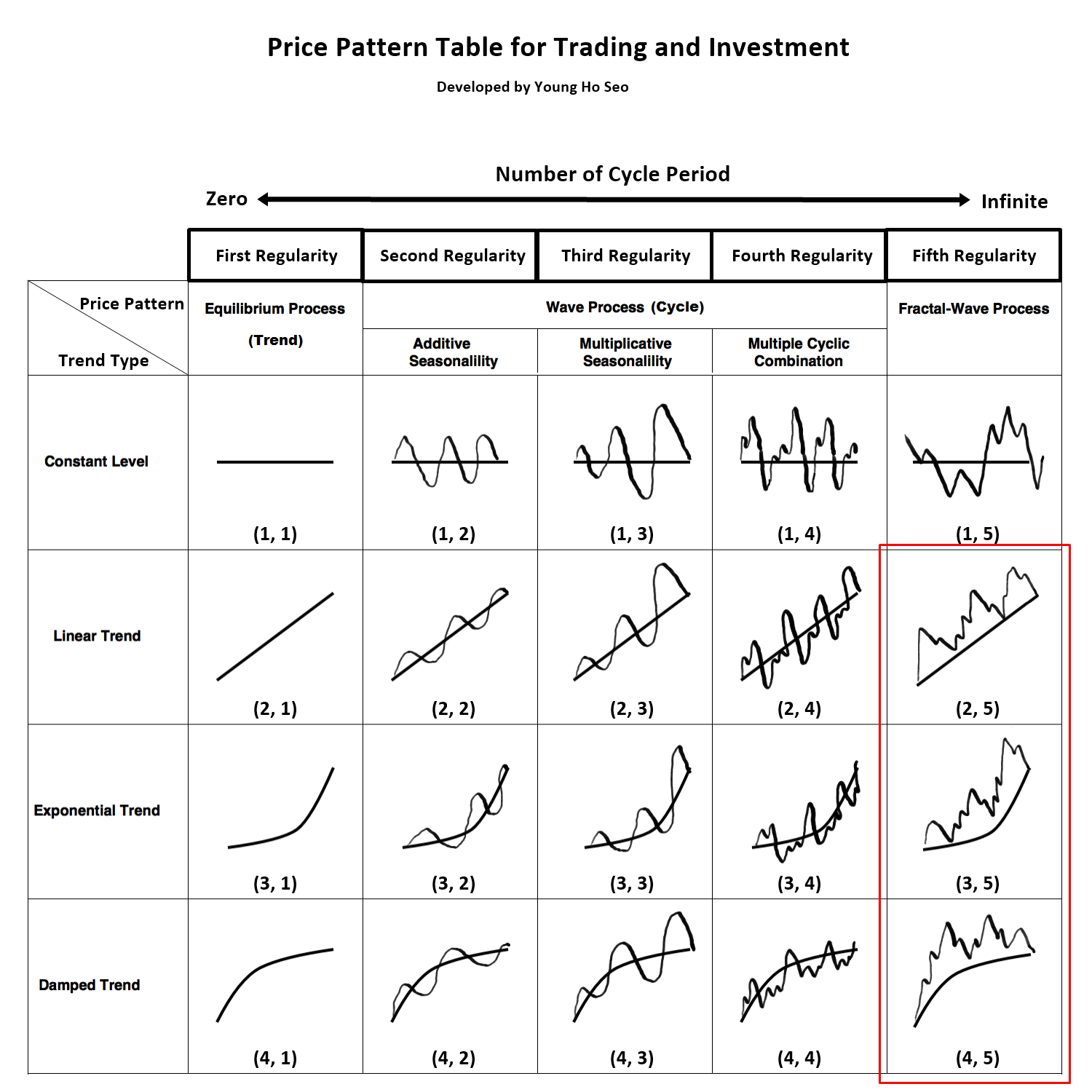
Figure 10-1: Equilibrium Fractal Wave process is corresponding to three price patterns (2, 5), (3, 5) and (4, 5) in the table.
Like Equilibrium Wave Process, Equilibrium Fractal-Wave process combines Equilibrium process with Fractal-Wave process (trend and fractal wave). Simply speaking, Equilibrium Fractal-Wave will show the trend patterns together with self-repeating wave patterns. Many financial prices series exhibit Equilibrium Fractal-Wave process in Stocks, Forex and Futures markets. In Chapter 8, we have shown how heartbeat and financial price series differ from each other even though they contain Fractal-Wave. In addition, in the analytical note, we have shown that in nature the building block of the fractal geometry can take many forms from line to square. In fact, this geometry is corresponding to Fractal dimension quantity. Here is one important question before proceeding. What would be the building block of the fractal geometry in the financial market?
We have already shown in Table 8-1 that Fractal Dimension of Financial market is between 1.2 and 1.5. This is close value to other Fractal geometry, whose building blocks are triangle. It is in the middle between line 1.0 and square 2.0 of fractal geometry. The basic building block of the fractal geometry in the financial market is most likely the triangle as shown in Figure 10-2. The triangle is made up from two price moves in the financial market. Since these triangles are propagating to reach the market equilibrium price, we can call these triangles as the equilibrium fractal wave. We have already covered the difference between Fractal wave and Equilibrium Fractal Wave. It depends on that price series has the horizontal patterns or not. For example, if the price series is fluctuating around the fixed mean, it is Fractal wave. If the price series is not bound to fixed mean and it has an open and unknown final destination, then it is Equilibrium Fractal Wave. In fact, for our financial trading, we need to concern more on equilibrium fractal wave than fractal wave.
To give you some idea on equilibrium fractal wave in the financial market, let us have some real world example using currency pairs. Regardless of how long the market goes on, the market can be described with few equilibrium fractal waves. For example, the financial prices series with 20 years of history can be described using two equilibrium fractal waves (Figure 10-2). Likewise, the price series with 2 weeks historical data can be described using two equilibrium fractal waves too (Figure 10-3). As you can see, they (Figure 10-2 and Figure 1—3) looks very similar. The main difference is that there are more jagged triangles inside the financial price series for 20 years comparing to the two weeks data.
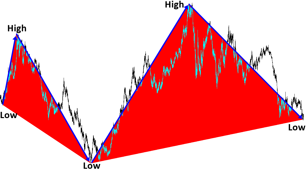
Figure 10-2: EURUSD twenty years’ historical data from 1992 to 2016.
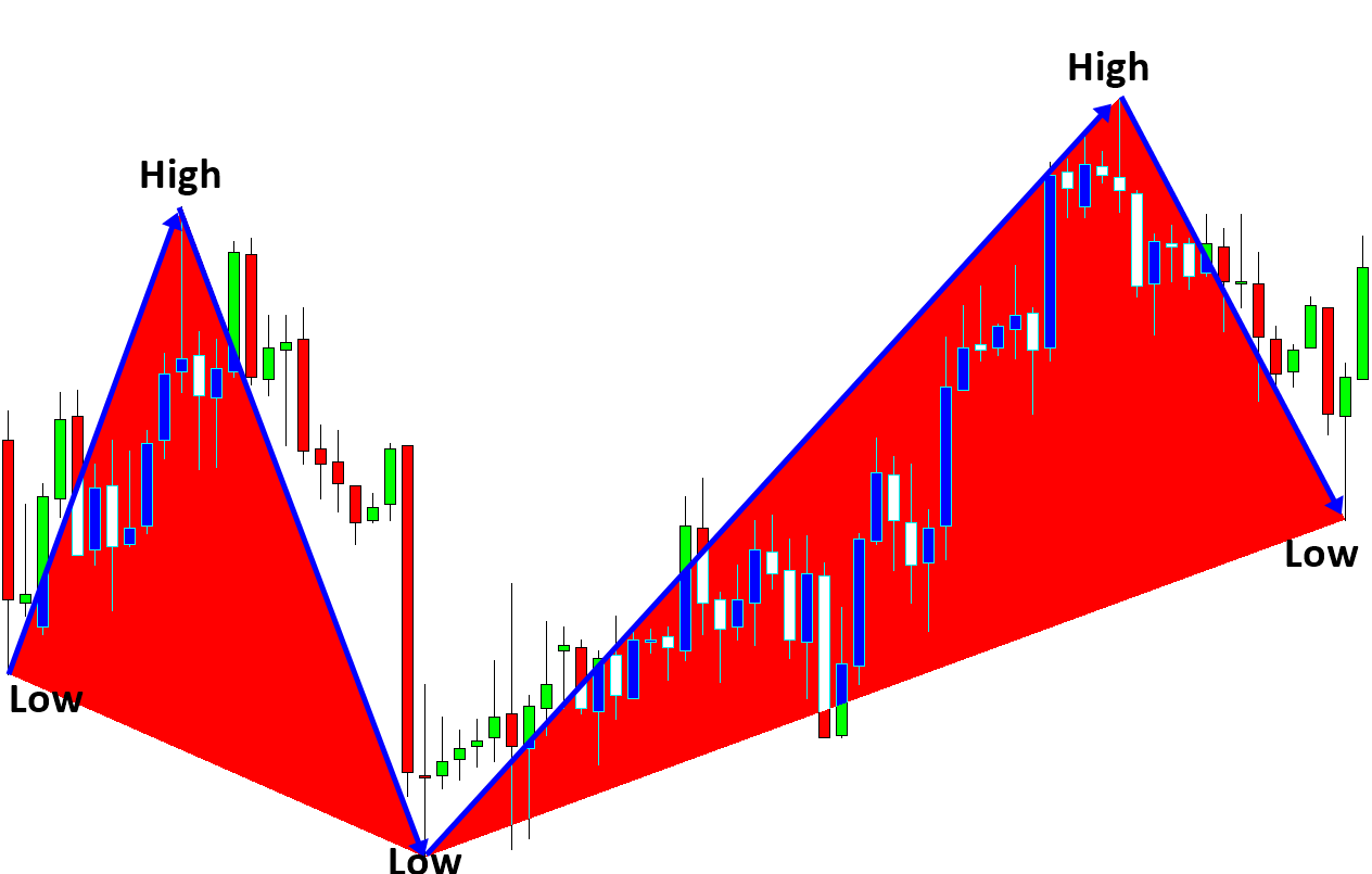
Figure 10-3: EURUSD two weeks historical Data from 2015 August 28 to 2015 September 16.
By definition, the building block of equilibrium fractal wave is equivalent to a triangle. In financial market, we have the loose self-similarity. This means that each triangle can have similar but different shapes. Since equilibrium fractal wave is made up from two price moves, one possible way to describe the shape of equilibrium fractal wave is by relating these two price moves. One can take the ratio of current price move to previous price move (Y2/Y1) to describe the shape of the equilibrium fractal wave typically.
Shape ratio of equilibrium fractal wave = current move in price units (Y2)/ previous move in price units (Y1).
Using Shape ratio, we can differentiate a specific shape of equilibrium fractal wave from other shapes. For example, Figure 10-6 shows two identical equilibrium fractal waves in their shape. Their shape can be considered as identical as their shape ratio is identical. Likewise, if the shape ratios of two equilibrium fractal waves are different, then two equilibrium fractal waves can be considered as non-identical shapes (Figure 10-7).
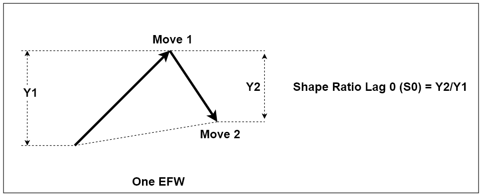
Figure 10-4: Structure of one ascending equilibrium fractal wave. It is made up from two price movements (i.e. two legs).
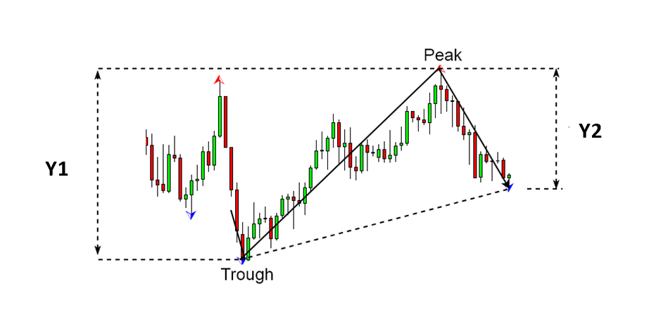
Figure 10-5: Building block of an equilibrium fractal wave in the candlestick chart.
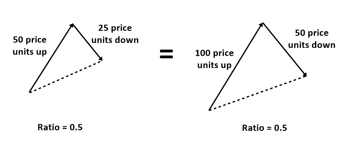
Figure 10-6: An example of two identical equilibrium fractal waves in their shape.
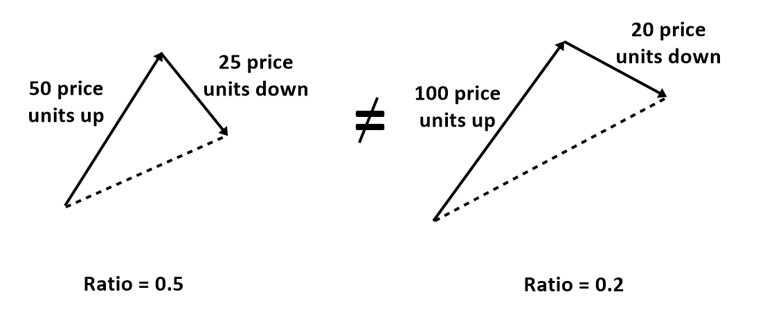
Figure 10-7: An example of non-identical equilibrium fractal waves in their shape.
When we want to describe price patterns with multiple triangles, we can have the multiple shape ratios. To avoid any confusion, we can just use the term “Lag” describe each shape ratio. For example, we can call the latest Shape ratio (Y3/Y2) as Shape Ratio Lag 0 (or S0). We can call the older one (Y2/Y1) as Shape Ratio Lag 1 (or S1). Figure 10-8 demonstrates this notation. This notation is useful when we have to study a pattern with more than two or three triangles.
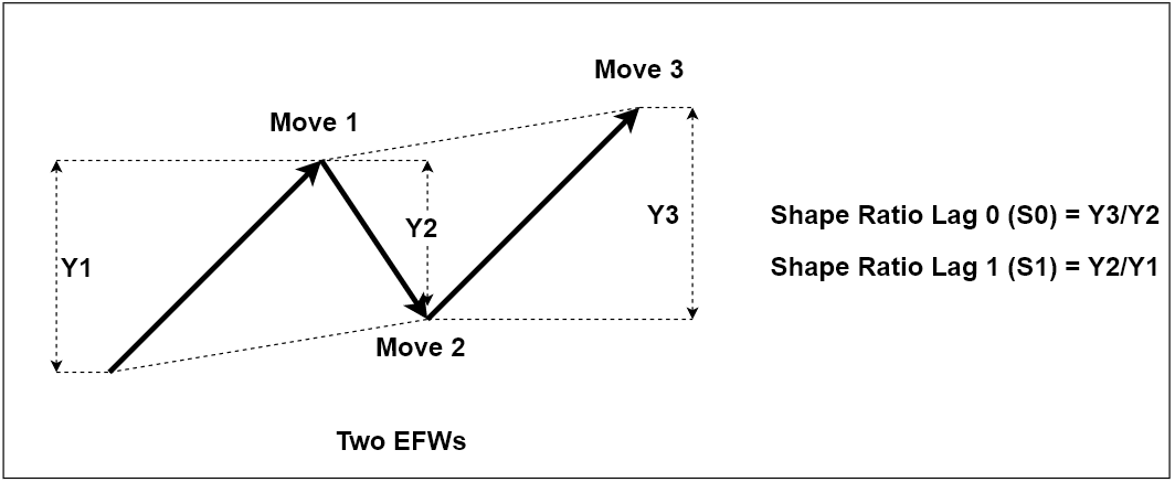
Figure 10-8: Shape ratios for two ascending Equilibrium Fractal waves
Besides, the Shape ratio, there is another important quantity useful to define the structure of the repeating patterns. That is Momentum Ratio. If Shape ratio measures the shape of each equilibrium fractal wave, then Momentum ratio measures the advancement of next wave in relation to the previous wave. In Momentum ratio, we measure the ratio between two-price movements in the same direction. For example, if the latest price movement was in the ascending direction, then the ratio is measured between the latest price movement of current wave and the first movement of the previous wave.
Momentum ratio of equilibrium fractal wave = latest price move of current wave in price units (Y3)/ first movement of previous wave in price units (Y1) where Y3 and Y1 are in the same direction.
Because we are measuring the ratio relating one wave to another, we need at least two equilibrium fractal waves to measure Momentum ratio. In Figure 10-9, we cannot measure Momentum ratio from one Triangle. In Figure 10-10, we can measure one Momentum ratio from two triangles. Likewise, in Figure 10-11, we can measure two Momentum ratios from three triangles. When we have multiple Momentum ratios, we can use the “Lag” term as before to differentiate each Momentum ratios. If you want to dig deeper on how to use this measurement, please check out the X3 Pattern notation at the end of this book. In fact, you could describe almost any EFW patterns in the Financial market using these two quantitiy.
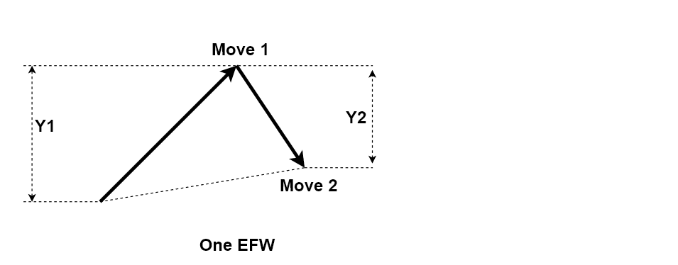
Figure 10-9: No Momentum ratio for one ascending Equilibrium Fractal wave
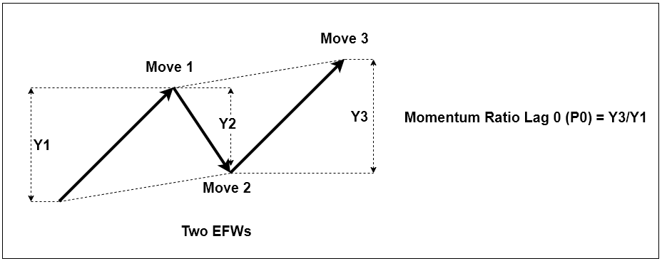
Figure 10-10: Momentum ratios for two ascending Equilibrium Fractal waves
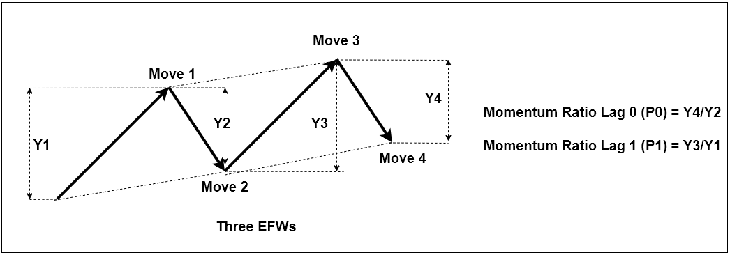
Figure 10-11: Momentum ratios for three ascending Equilibrium Fractal waves
To use Equilibrium Fractal Wave for our trading, we have to understand the characteristics of equilibrium fractal wave. In this book, we outline the five most important characteristics for your trading. When you trade with a single equilibrium fractal wave or multiple of equilibrium fractal waves (i.e. Elliott wave or harmonic patterns), you will find out that the trading strategies are based on one or few of these characteristics.
The first characteristic of equilibrium fractal wave is the repeatability. While the price is moving to its equilibrium price level, we observe the zigzag path of the price movement. After extensive price rise, the price must fall to realize the overvaluation of the price. Likewise, after extensive price fall, the price must rise to realize the undervaluation of the price. This price mechanism builds the complex zigzag path of the price movement. During the zigzag path, the price shows the four possible triangle shapes as shown in Figure 10-12. These four equilibrium fractal waves are the mirrored image of each other. Therefore, they are the fractal. The complex price path in the financial market is in fact the combination of these four equilibrium fractal waves in alternation. Whenever the price needs to move on to the equilibrium level, the price will travel in the zigzag path through the combination of these four equilibrium fractal waves in alternation.
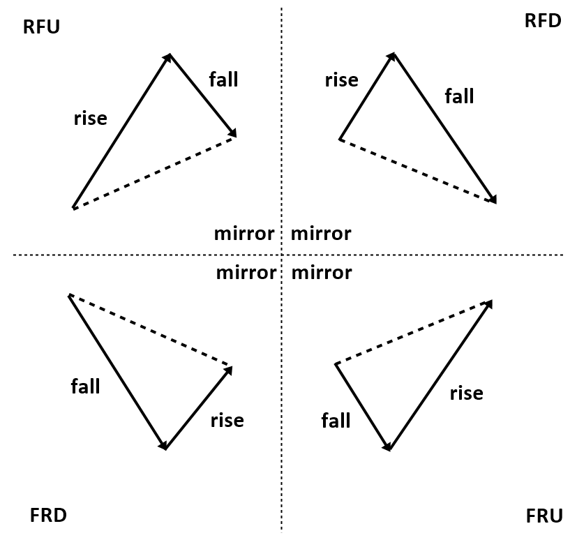
Figure 10-12: Equilibrium fractal wave in the Zig Zag price path where RFU = Rise Fall UP pattern, RFD = Rise Fall Down pattern, FRD = Fall Rise Down pattern and FRU = Fall Rise Up pattern.
The second characteristic of equilibrium fractal wave is that equilibrium fractal wave can be extended to form another bigger equilibrium fractal wave as shown in Figure 10-13. During economic data release or market news release, financial market can experience a volatility shock. When market experiences the volatility shock, the last leg of equilibrium fractal wave can extend to adapt the shock introduced in the market. Even after the extension, the equilibrium fractal wave still maintains its fractal geometry, the triangle. Hence, the fractal nature of financial market is unbreakable. This price extension often determines the reversal or breakout movement around the important support and resistance levels. One possible way of trading with this second characteristic is to trade on the potential size of equilibrium fractal wave. In the case of reversal, we are betting on that the size of wave will be small. In the case of breakout, we are betting on that the size of wave will be big. This characteristic is also the basis for the straddle trading strategy during the important economic data release.
![]()
Figure 10-13: Illustration of price transformation (extension) from path 1 to path 2 to meet new equilibrium price due to an abrupt introduction of new equilibrium source in the financial market.
Third characteristic of equilibrium fractal wave is that smaller equilibrium fractal waves can combine to form a bigger Equilibrium Fractal Wave. Imagine, when the equilibrium fractal wave is propagating, it will start with smaller equilibrium fractal waves first. After the appearance of the several equilibrium fractal waves, we can draw the bigger equilibrium fractal wave by joining these smaller waves. These kinds of jagged patterns are repeatedly found in the financial market as shown in Figure 10-14. This third characteristic is often used by a professional trader to improve the predictability of the financial market. For example, instead of puzzling with a set of small equilibrium fractal waves, it is much more accurate to puzzle with both small and big equilibrium fractal waves together to predict the market direction. If you want to become a successful trader, you will need a discipline on how to combine small and big equilibrium fractal waves for your trading. Of course, later, we will show you how to improve your trading performance using this principle.
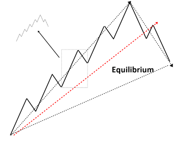
Figure 10-14: Pictorial representation of jagged (superimposed) equilibrium fractal wave with a linear trend.
The fourth characteristic of equilibrium fractal wave is the infinite scales. The infinite scales mean that you will see the similar patterns repeatedly in the price series while their sizes are keep changing. The repeating pattern can come in any size from small to large. For example, if we stack the varying size of equilibrium fractal waves with the particular shape ratio, then literarily we can stack the infinite number of triangle as shown in Figure 10-15. This implies the infinite number of cycle periods in Figure 3-3 and Figure 3-4. This is exactly why “Equilibrium Fractal-Wave” process is much harder to be handled by traditional technical indicators because they were not designed to deal with the infinite scaling problem most of time.
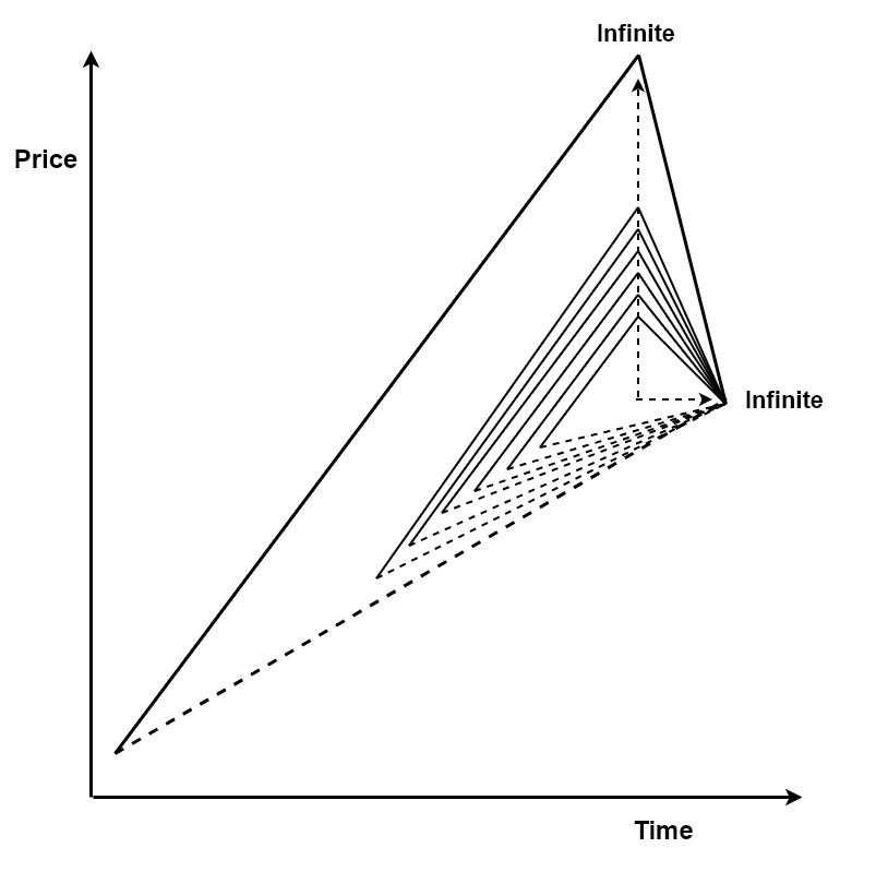
Figure 10-15: Infinite number of stacked triangles.
The fifth characteristic of equilibrium fractal wave is the loose self-similarity (heterogeneity). In nature, it is easy to find the strict self-similarity. However, we can only expect the loose self-similarity in the financial market due to the highly diverse players, participating in the market. Even though all the equilibrium fractal waves will have the triangular form, their shape ratios will be different. For example, if we display all shape ratios in price series, we will expect the different shape ratios to its adjacent one (Figure 10-16). This does not mean that we will never have the similar or identical shape ratios in history. In fact, we get lots of them repeating in the history. For example, we get to see the shape ratio of 0.618 all the time in the financial market. However, we are just saying that the same shape ratios will not often come in the successive manner. This heterogeneous characteristic also implies that the financial market have some shapes more frequently occurring than some other shapes. This also has an important implication for our trading. Imagine that we have a financial market with three shape ratios 0.450, 0.850 and 1.300. We only found the shape ratio 0.450 and 1.300 repeated ten times in the historical data whereas the shape ratio 0.850 repeated 100 times in the historical data. Which shape ratio shall we trade with? Of course, we will trade with the ratio 0.850. Likewise, last hundreds years, traders had a solid belief in using the Fibonacci ratios like 0.618, 0.382 and 1.618 for their trading. This belief is based on the assumption that the Fibonacci ratios 0.618, 0.382 and 1.618 occurs more frequently comparing to other non-Fibonacci ratios like 0.567, 0.855, 1.333, etc in the financial market. This loose self-similarity (heterogeneity) is the rationale behind the Fibonacci ratio analysis and other Fibonacci ratio based strategies like Elliott Wave and Harmonic Pattern. The main idea is that, among many shape ratios, we need to choose the most frequently occurring shape ratio for our trading.
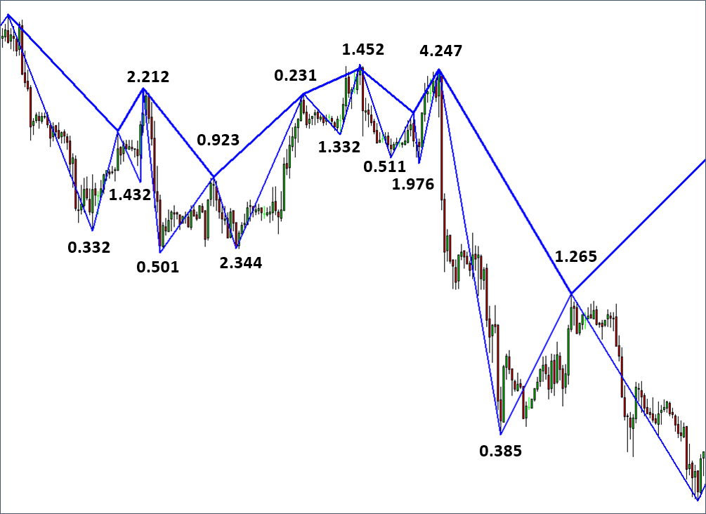
Figure 10-16: Equilibrium fractal waves with different shape ratios.
Each equilibrium fractal wave can be combined to form the patterns that are more complex. Several popular tradable patterns can be derived by combining several equilibrium fractal waves. For example, Harmonic patterns are typically made up from three equilibrium fractal waves. Impulse Wave 12345 pattern in Elliott Wave Theory is typically made up from four equilibrium fractal waves. Corrective Wave ABC pattern in Elliott Wave Theory is made up from two equilibrium fractal waves. Like the case of Elliott Wave patterns and Harmonic patterns, some derived patterns can have some definite number for equilibrium fractal wave for the defined patterns. However, there are some derived patterns does not have the definite number of equilibrium fractal wave. For example, rising wedge, falling wedge and triangle patterns does not require the definite number of equilibrium fractal wave. Rising wedge, falling wedge and triangle patterns are envelops connecting highs and lows of each equilibrium fractal wave.
| EFW Derived patterns | Number of equilibrium fractal waves | Number of points |
| ABCD pattern | 2 | 4 |
| Butterfly pattern | 3 | 5 |
| Gartley pattern | 3 | 5 |
| Impulse Wave 12345 | 4 | 6 |
| Corrective wave ABC | 2 | 4 |
| Falling wedge pattern | Not defined | Not defined |
| Rising wedge pattern | Not defined | Not defined |
| Symmetric triangle | Not defined | Not defined |
| Ascending triangle | Not defined | Not defined |
| Descending triangle | Not defined | Not defined |
Table 10-1: List of derived patterns for trader from equilibrium fractal waves
The properties of these derived patterns remain identical to single equilibrium fractal wave because the derived patterns are also fractals by nature. Therefore, the derived patterns are repeating in different scales. For example, the size of butterfly pattern detected in EURUSD today will be different to the butterfly pattern detected 1 month ago. In addition, the size of butterfly pattern detected in EURUSD will be different to the butterfly pattern detected in GBPUSD. The detected patterns can have slightly different shape ratios too. It is also possible to have nested patterns inside larger patterns. For example, we can have a small bullish butterfly pattern inside the greater bullish butterfly pattern. Likewise, we can have a nested bullish Impulse Wave 12345 pattern inside greater bullish Impulse Wave 12345 pattern. Another important point about these derived patterns is that they will serve for the price to propagate in the direction of the market equilibrium. The formation of the repeating patterns will typically guide the price to the end of the equilibrium price. Some derived patterns like Harmonic Patterns can pick up the trend reversal. Some patterns like impulse wave 1234 can help you to predict trend continuation. Therefore, these derived patterns provide good clue about trading direction for us. Presence of these derived patterns can represent the existence of fifth regularity, equilibrium Fractal-Wave process in the financial price series.
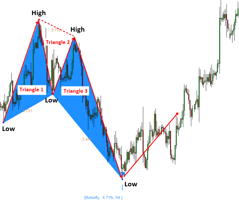
Figure 10-17: Butterfly pattern formed in EURUSD H4 timeframe.
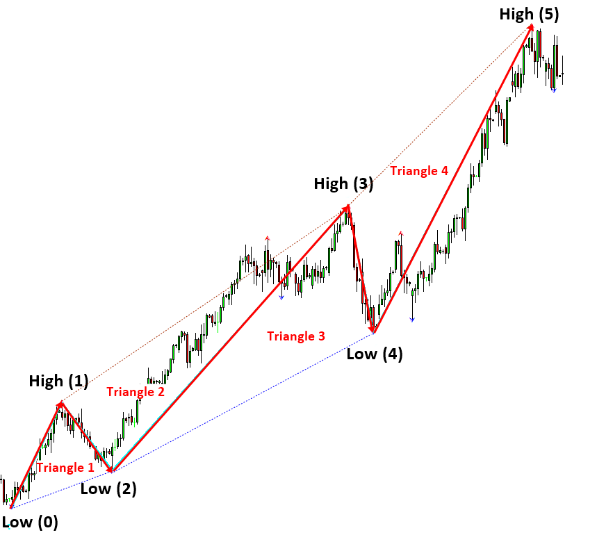
Figure 10-18: Impulse Wave 12345 pattern formed in EURUSD D1 timeframe.
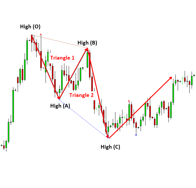
Figure 10-19: Corrective Wave ABC pattern formed in EURUSD D1 timeframe.
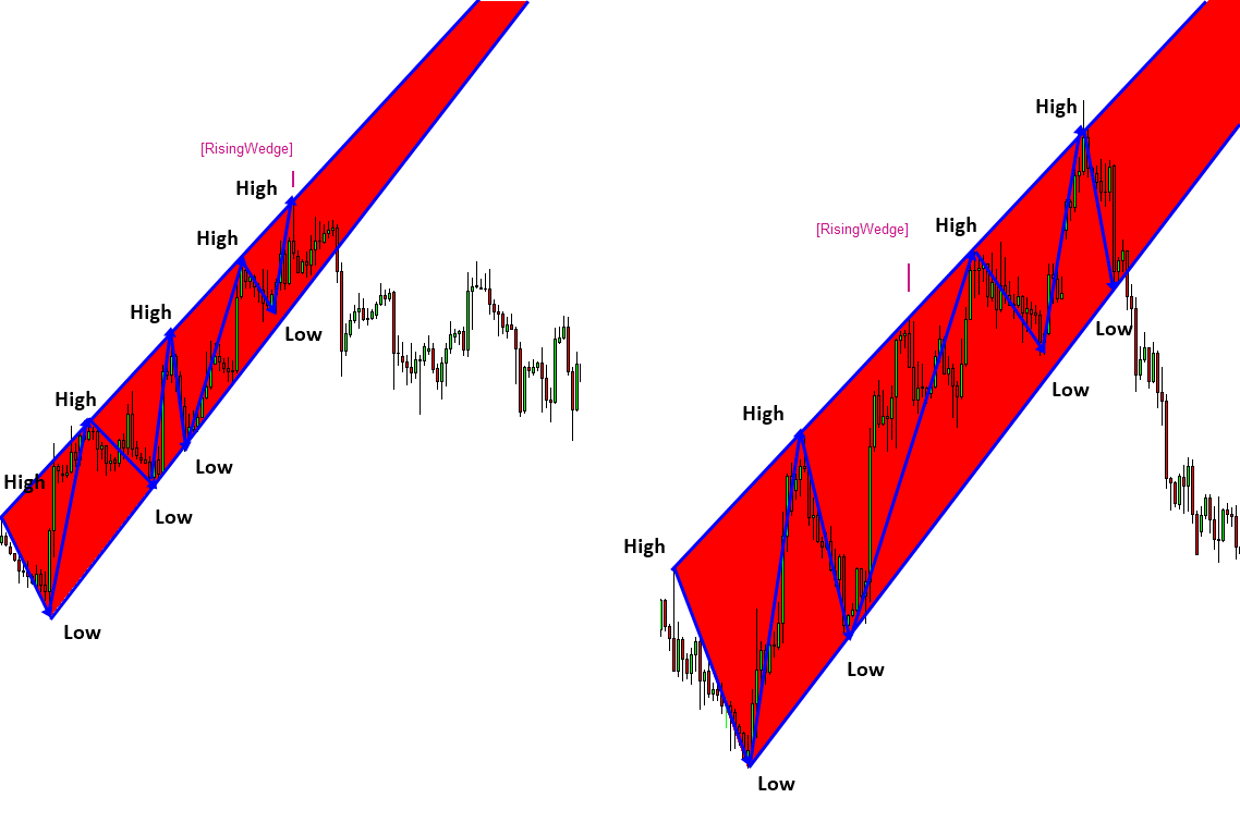
Figure 10-20: Rising Wedge pattern A (left) and another Rising Wedge pattern B (right) formed in EURUSD H4 timeframe.
Some More Tips about Equilibrium Fractal-Wave Process in Forex Trading
The Equilibrium Fractal-Wave Process is a sophisticated concept in Forex trading that combines elements of fractal theory, wave analysis, and equilibrium states to identify trading opportunities. This approach is rooted in the idea that market prices exhibit fractal characteristics and follow wave-like patterns that tend to move towards an equilibrium state.
Key Concepts
Fractal Pattern in Forex Trading:
Fractal Pattern: These are recurring patterns that are self-similar across different scales. In Forex trading, fractal pattern are used to identify potential reversals in the market.
Wave Theory:
Elliott Wave Theory: This theory posits that market prices move in predictable wave patterns consisting of impulsive waves (trending in the direction of the main trend) and corrective waves (moving against the main trend). Traders use this to predict future price movements.
Harmonic Patterns: These are specific price patterns that align with Fibonacci ratios to predict potential price reversals. Examples include the Gartley pattern, Butterfly pattern, and Bat pattern.
Equilibrium State:
Market Equilibrium: This refers to the point where the supply and demand for a currency are balanced, leading to stable prices. In trading, equilibrium can be identified using various indicators, such as moving averages, Bollinger Bands, or support and resistance levels.
Integrating Fractals, Waves, and Equilibrium
The Equilibrium Fractal-Wave Process in Forex trading integrates these three concepts to provide a comprehensive analysis of market movements:
Identifying Fractal Pattern:
Use fractal Pattern indicators to detect recurring patterns and potential reversal points on different time frames. This helps in recognizing the underlying structure of the market.
Wave Analysis:
Apply Elliott Wave Theory or harmonic patterns to understand the larger wave structure of the market. This aids in identifying the main trend and its corrective phases.
Finding Equilibrium:
Use indicators like moving averages, Bollinger Bands, and Fibonacci retracements to identify equilibrium points where the market might stabilize before the next move. Support and resistance levels also play a crucial role in determining equilibrium.
Practical Application in Forex Trading
Pattern Recognition:
Look for fractal patterns that coincide with wave patterns to pinpoint high-probability entry and exit points. For example, a fractal reversal at the end of a corrective wave might indicate the start of a new impulsive wave.
Multiple Time Frame Analysis:
Analyze fractal patterns and wave structures across multiple time frames to confirm trading signals. A fractal on a lower time frame within a larger wave pattern on a higher time frame can provide strong confirmation.
Risk Management:
Use equilibrium points to set stop-loss and take-profit levels. For example, placing a stop-loss just beyond a key support or resistance level identified through equilibrium analysis can help manage risk effectively.
Algorithmic Trading:
Develop automated trading systems that incorporate fractal, wave, and equilibrium analysis. These systems can continuously scan the market for patterns and execute trades based on predefined criteria.
Advantages and Limitations
Advantages:
- Comprehensive Analysis: Combines multiple technical analysis methods for a robust market analysis.
- Predictive Power: Enhances the ability to predict future price movements by understanding market structure and behavior.
- Flexibility: Can be applied to various time frames and trading styles.
Limitations:
- Complexity: Requires a deep understanding of fractal theory, wave analysis, and equilibrium concepts.
- Subjectivity: Interpretation of fractals and wave patterns can be subjective and may vary between traders.
- Market Conditions: May not perform well in highly volatile or erratic market conditions where patterns are less predictable.
Conclusion
The Equilibrium Fractal-Wave Process is a powerful approach to Forex trading that integrates fractal patterns, wave theory, and market equilibrium concepts. By combining these elements, traders can gain deeper insights into market behavior and improve their ability to identify profitable trading opportunities. However, mastering this approach requires extensive knowledge and practice, as well as a disciplined and analytical trading mindset.
About this Article
This article is the part taken from the draft version of the Book: Scientific Guide To Price Action and Pattern Trading (Wisdom of Trend, Cycle, and Fractal Wave). This article is only draft and it will be not updated to the completed version on the release of the book. However, this article will serve you to gather the important knowledge in financial trading. This article is also recommended to read before using Price Breakout Pattern Scanner, Advanced Price Pattern Scanner, Elliott Wave Trend, EFW Analytics and Harmonic Pattern Plus, which is available for MetaTrader 4 and MetaTrader 5 platform.
Below is the landing page for Price Breakout Pattern Scanner, Advanced Price Pattern Scanner, Elliott Wave Trend, EFW Analytics and Harmonic Pattern Plus. All these products are also available from www.mql5.com too.
https://algotrading-investment.com/portfolio-item/price-breakout-pattern-scanner/
https://algotrading-investment.com/portfolio-item/advanced-price-pattern-scanner/
https://algotrading-investment.com/portfolio-item/elliott-wave-trend/
https://algotrading-investment.com/portfolio-item/equilibrium-fractal-wave-analytics/
https://algotrading-investment.com/portfolio-item/harmonic-pattern-plus/
Related Products