Fractal-Wave Process
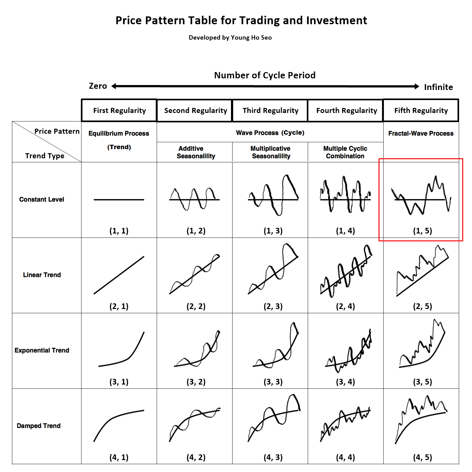
Figure 8-1: Fractal-Wave process is corresponding to price pattern (1, 5) in the table.
Fractal-Wave process is the representation of the Fractal geometry in the time dimension. Fractal geometry is made from a repeating pattern at many different scales. Simply speaking it is repeating patterns with varying size. Fractal geometry can be a self-similar pattern with the strictly same patterns across at every scale. Or if the pattern loosely matches to the past one, this can be still considered as fractal geometry. We call this as near self-similarity against the strict self-similarity. Many examples of Fractal geometry can be found in nature. Snowflakes, coastlines, Trees are the typical example of the Fractals geometry in space. Fractal-Wave is the fractal geometry generated in time dimension. Just like Fractal Geometry can be described by self-similar patterns. Fractal-Wave can be described by self-similar patterns repeating in time. The concept of Fractal-Wave can be illustrated well by Weierstrass function.
Loosely speaking, Weierstrass function is the cyclic function generated from infinite number of Cosine functions with different amplitude and wavelength. By combining infinite number of Cosine functions, it can generate a complex structure repeating self-similar patterns in different scales. This is a typical synthetic example of Fractal-Wave patterns with strict self-similar patterns. We present this function to help you to understand the properties of the self-similar process. The real world financial market shows the loose fractal geometry. They do not repeat in the identical patterns in shape and in size. The repeating patterns are similar to each other up to certain degree. Since Weierstrss function is the synthetic example for the strict fractal geometry, reader should note that Weierstrss function does not represent the real world financial market.
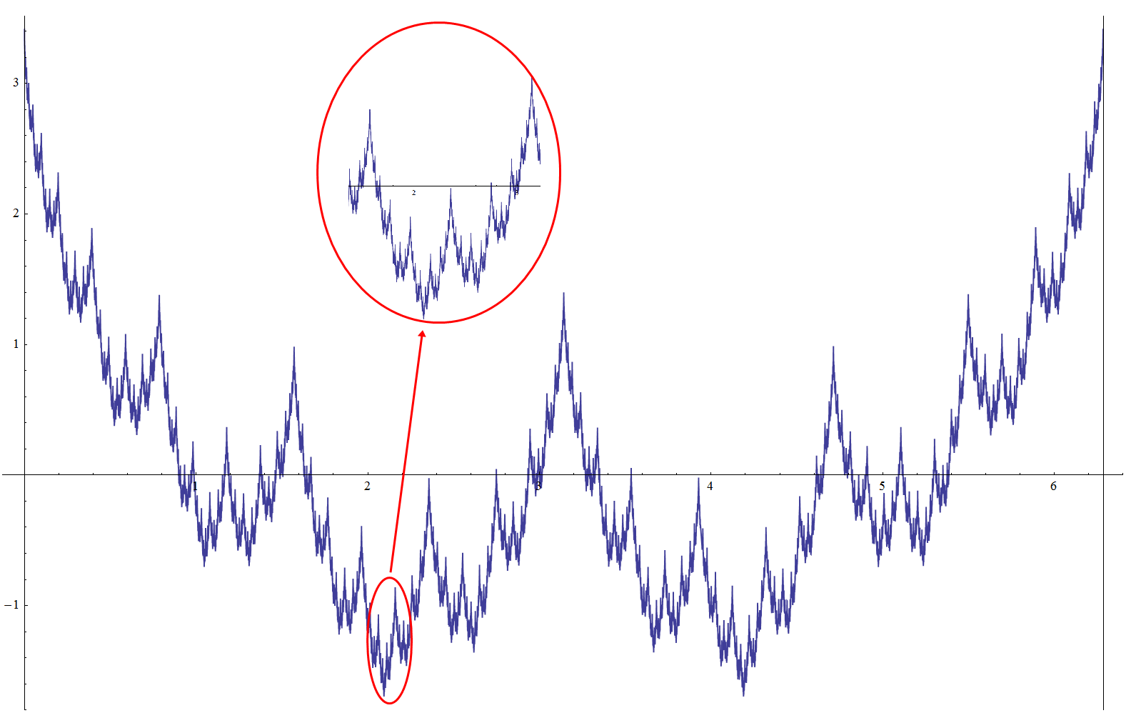
Figure 8-2: Weierstrass function to give you a feel for the Fractal-Wave process. Note that this is synthetic Fractal-Wave process only and this function does not represent many of real world cases.
In the real world application, Fractal-Wave process appears with the near self-similar patterns most of time. Therefore, detecting them is not easy. The Heart Beat Rate signal is one typical example of the Fractal-Wave process in nature (Figure 8-3 and Figure 8-4). If we zoom in on a subset of time series, we can see the apparent self-similar patterns. In Financial Market, Fractal-Wave process occurs frequently but the market typically shows the near self-similarity too. In terms of pattern shape, the financial market and Heart beat rate signal are different because their underlying pattern generating dynamics inside human organ and crowd behaviour are substantially different.
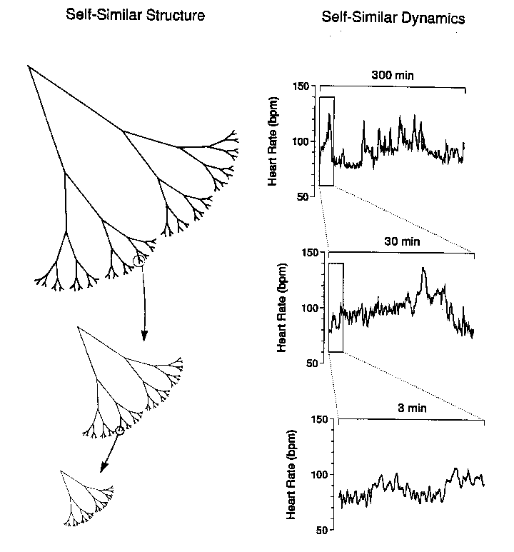
Figure 8-3: Self-similar process in Heart Beat rate (Goldberger et al, 2000).
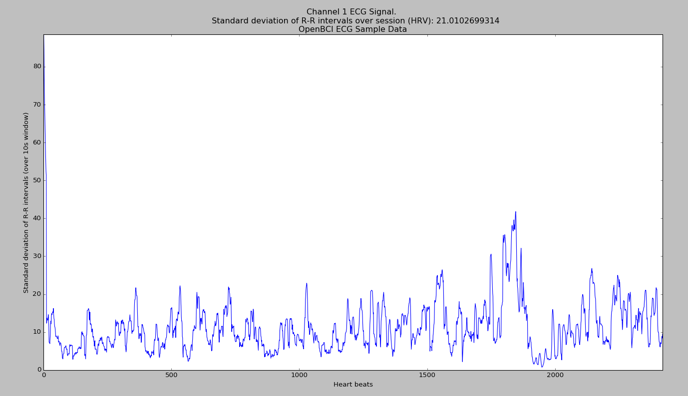
Figure 8-4: Continuous Heart Beat time series.
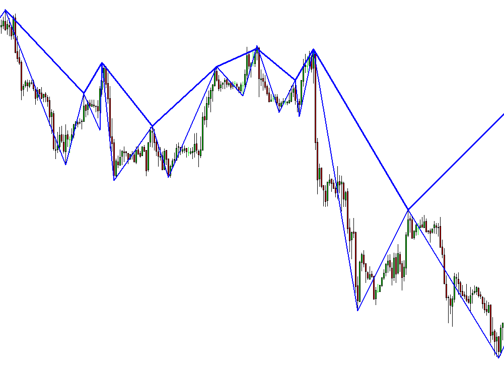
Figure 8-5: Self-similar geometry in EURUSD daily series.
Fractal-Wave process is the basis for many popular trading strategies like Elliott Wave, Harmonic patterns, triangle and wedge patterns. However, these trading strategies were not well connected to existing science in the past. This was one of the important motivation for myself to step up to write and to connect these trading strategies into existing science. Most of time, day traders were referencing that these strategies will work because market repeats themselves. For me, this explanation would be not enough before I make the full time commitment on them.
Therefore, I had to do a lot of research to find the origin of these trading strategies and to see real value behind them. From my research, most likely, the repeating patterns in these strategies come from Fractal-Wave. I was very happy initially until I found that there is big difference between the underlying concepts of these trading strategies and Fractal-wave itself.
To see the difference, you might compare the heart beat signal and EURUSD price series in Figure 8-4 and Figure 8-5. You could also compare the heartbeat signal and S&P 500 series in Figure 8-6. With heart beat signal in Figure 8-4, you might think that it would look similar to Stock or Forex market data but different in some ways. If you felt this way, you are very correct. Here is the main difference.
Heartbeat signal seems to have fixed mean or horizontal patterns as we described in Stationary process in Chapter 5. However, EURUSD price series or S&P 500 series do not show any noticeable horizontal patterns. With human, the heartbeat increases dramatically to get more blood out during intensive activity like sprinting, but they must come back to normal range to maintain our life. Naturally, this makes up the horizontal patterns as we described in Stationary process. On the other hands, the operational range of the financial market does not have to create the horizontal patterns as if heartbeat does. Firstly, financial market is designed to grow or decline with time (Figure 8-6). Secondly, the underlying fundamental drives the rise and fall of the financial market (Figure 8-6) towards unknown destination.
With human, we know that our heartbeat rate must be kept between 60 and 100 times per minute. While you are a living man, this normal range is the destination of your heartbeat rate most of time. It is very predictable that your heartbeat will come back to 80 times per minute once it hits 130 times per minute. In the financial market, the final destination is not known and open. Even if S&P500 hits 3000 points tomorrow, we are not sure if it would even come back to 1000 points next year or ever. Hence, we are talking about similar but very different type of Fractal-Wave. Fractal wave alone can not explain the difference between these two. In the past, many day traders were having misleading picture between fractal wave and these trading strategies because no one or no literature attempted to give clear or easy explanation on them. This was another motivation for me to write this book too.
The open and unknown destination of the financial market is there because the underlying fundamental drives the market towards the price level, at which majority of people think it is most reasonable. In another words, market will move towards the equilibrium price. We have covered this in Equilibrium process in Chapter 8. Financial market is not only made up from Fractal-Wave but with Equilibrium process too. Hence, this is why financial market is different from heartbeat series although both have fractal wave in them. We have just pinned down the important concept of Equilibrium Fractal Wave process. In next two chapters, we will take you to the details of Equilibrium Wave process and Equilibrium Fractal Wave process to give you the complete and systematic view of the trading strategy and financial market.
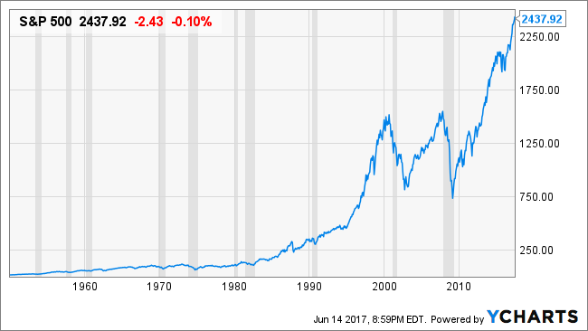
Figure 8-6: S&P 500 growth last 70 years.
Analytical Note
In the Fractal Geometry, two important quantifiable properties are fractal dimension and self-similarity. Fractal dimension is a measure of how much an N dimensional space is occupied by an object. For example, a straight line have dimension of 1 but a wiggly line has a dimension between 1 and 2. More precisely, their Fractal Dimension can be expressed as Log (N)/Log (r) where N = number of self-similar pieces and r = linear scale factor. Now to illustrate the concept, we will present the four cases from dimension 1 to 2. If we reduce size of straight line by linear scale factor r = 2, then then we get two self-similar piece, N = 2. Therefore, the dimension of the straight line is 1.
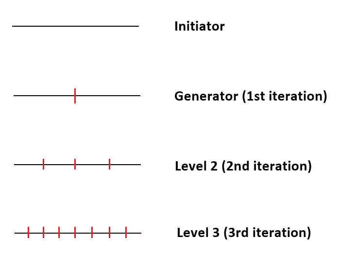
Figure 8-7: Iteration of self-similar process for straight line (Dimension = 1).
Likewise, if we remove the middle third of the straight line and replace it with two lines with the same length, then we get the first iteration of the Koch Curve. In this example, for the linear scale factor r = 3, we get the four self-similar pieces. Therefore, the dimension of Koch Curve is 1.26816 = Log (4) / Log (3).
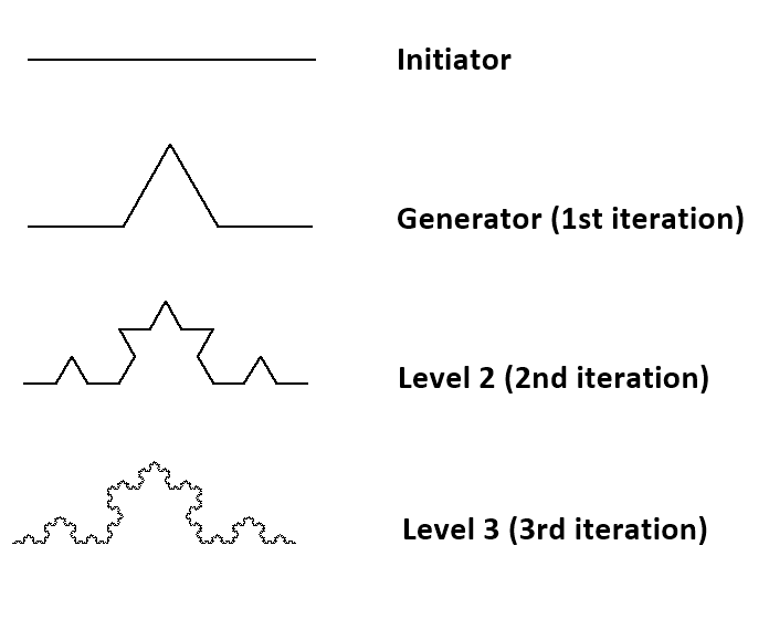
Figure 8-8: Iteration of self-similar process for Koch Curve (Dimension = 1.26816).
Sierpinski Triangle is another good example of Fractal Geometry. If we connect the mid points of the three side inside an equilateral triangle, then we get 3 equilateral triangles inside the first equilateral triangle. Note that we do not count the resulting upside down triangle as a self-similar piece. In this case, the linear scale factor r is 2 since generated triangle have the half of the width and height. The Fractal dimension D = 1.585 = Log (3)/ Log (2).
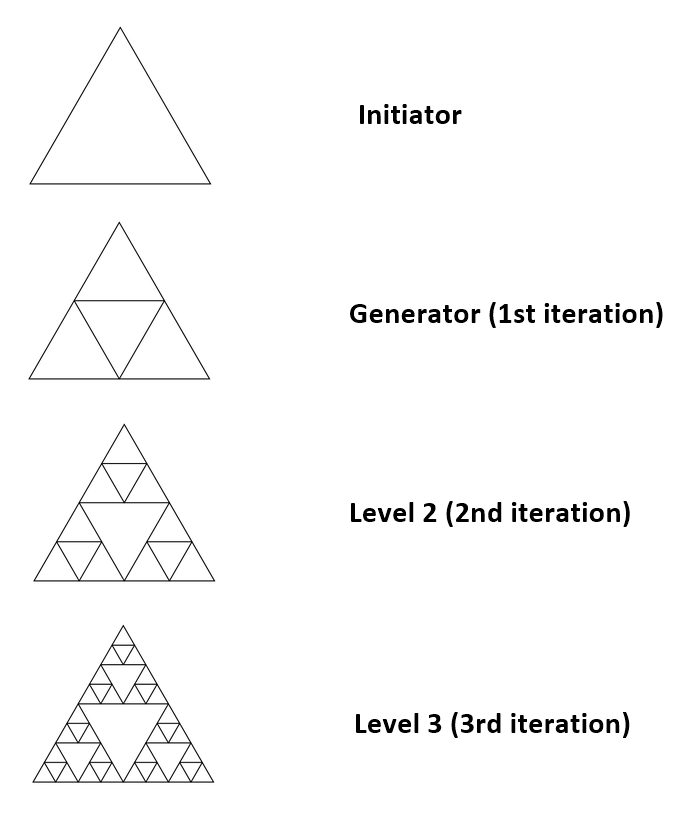
Figure 8-9: Iteration of self-similar process for Sierpinski Triangle (Dimension = 1.585).
Finally consider a square. For the linear scale factor r = 2, we will get four squares inside the first one. Therefore, our fractal dimension for a square is D = 2 = Log (4) / Log (2). Even we make the linear scale factor r = 3, we still get the same Fractal dimension D = 2 = Log (9) / Log (3). As we have illustrated in the four examples, Fractal Dimension generalize the topological integer dimensions to a fraction. Higher the fractal dimension means that the fractal geometry to occupy more space in the dimension. Therefore, a square have the Fractal Dimension 2 as the smaller square fits larger one without leaving any empty space. If our fractal geometry is kept removing space, then we could get the Fractal Dimension less than 1 too.
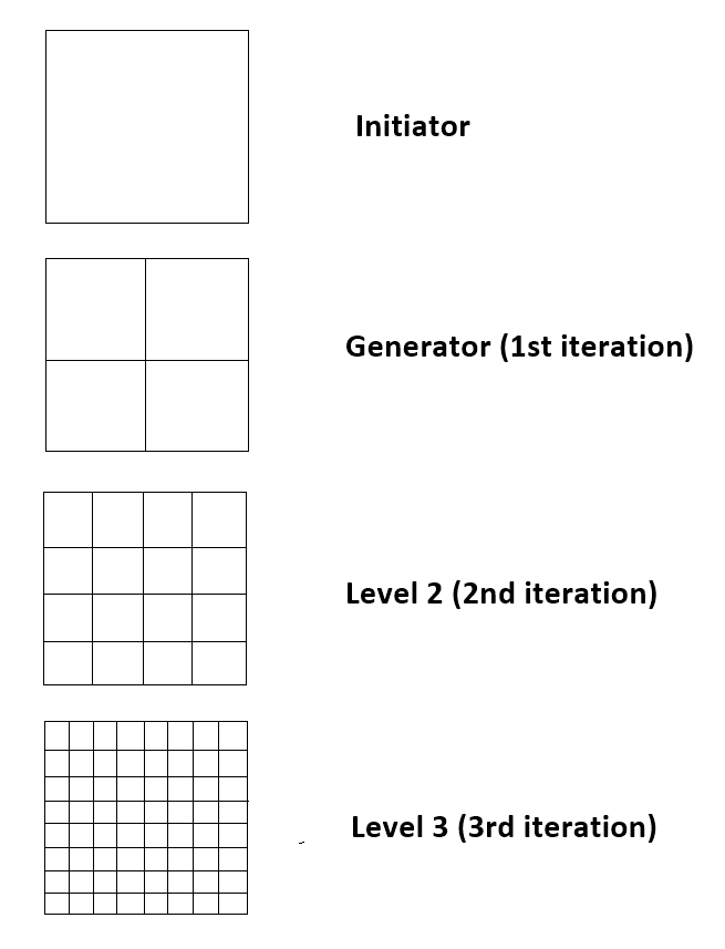
Figure 8-10: Iteration of self-similar process for square (Dimension = 2).
If the fractal geometry is known like our four examples above, then calculating Fractal dimension for that fractal geometry is straightforward. However, in many practical applications, the self-similar patterns are not strict and difficult to identify. For example, the rocky coastline have the fractal dimension with near self-similarity. In such a case, we can still calculate the Fractal Dimension using some iterative methods. To calculate the length of wiggly line in the rocky coastline, one can measure the length by counting how many times a measuring stick with a known length can be fitted along the coastline: L(s) = N x s. By plotting the length of the coastline versus the length of the measuring stick on a double logarithmic scale, one obtains the following equations to calculate the Fractal Dimension for the coastline: Log (L (s)) = (1-D) Log (s) + constant. Therefore, the measured slope can be used to calculate the Fractal Dimension. For example, Figure 8-11 shows the plot of the length of the coastline versus the length of the measure stick on double logarithmic scale for different countries. For Great Britain, the Fractal dimension can be calculated as D = 1 – (-0.24) = 1.24. Higher the Fractal Dimensions means greater the jaggedness or non-smoothness of the coastline.
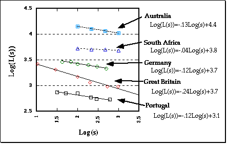
Figure 8-11: Measured slope of Log (L (s)) versus Log (s) for the coastline of the five countries including Australia, South Africa, Germany, Great Britain and Portugal. (Source: Vanderbilt University Webpage, http://www.vanderbilt.edu)
Calculating the Fractal Dimension for financial market data is not easy because it is harder to use such a measuring stick to measure the length of the line. Alternatively one might use Hurst Exponent (H) to calculate Fractal Dimension (D = 2–H) for a rough estimation of Fractal Dimension. Table 8-1 shows Hurst Exponents for several international Stock and Currency pairs. Using the relationship between Hurst Exponent and Fractal dimension, we can find that Fractal Dimension for many stock index lies somewhere between 1.2 and 1.5. Of course, this is very rough estimation only with some margin of error. Considering our four example earlier, we can imagine that the complexity of the financial price series might lies between Koch Curve and Sierpinski Triangle.
| Financial Instrument | Start Time | End Time | FDI for D1 Timeframe |
| EURUSD | 2006 7 21 | 2018 2 9 | 1.48 |
| GBPUSD | 2006 7 20 | 2018 2 9 | 1.43 |
| USDJPY | 2006 7 21 | 2018 2 9 | 1.47 |
| AUDUSD | 2006 7 21 | 2018 2 9 | 1.47 |
| USDCAD | 2006 7 24 | 2018 2 9 | 1.46 |
| NZDUSD | 2006 7 20 | 2018 2 9 | 1.49 |
| EURGBP | 2006 7 14 | 2018 2 9 | 1.48 |
| USDCHF | 2006 7 20 | 2018 2 9 | 1.45 |
| IBM Corporation | 2005 5 19 | 2018 2 9 | 1.46 |
| Intel Corporation | 2005 7 8 | 2018 2 9 | 1.45 |
| Microsoft Corporation | 2005 6 29 | 2018 2 9 | 1.39 |
| Citi Group Inc. | 2005 7 6 | 2018 2 9 | 1.42 |
| Walt Disney Company | 2005 6 9 | 2018 2 9 | 1.40 |
| General Electric Corporation | 2005 7 13 | 2018 2 9 | 1.44 |
| Coca Cola Company | 2005 7 11 | 2018 2 9 | 1.45 |
| Boeing Company | 2005 5 20 | 2018 2 9 | 1.36 |
| Average | 1.44 | ||
| Standard deviation | 0.04 | ||
| 95% Upper Confidence Interval | 1.51 | ||
| 95% Lower Confidence Interval | 1.37 |
Table 8-1: Fractal Dimension index for D1 Timeframe
Some More Tips about Fractal Wave Process in Forex Trading
The Fractal-Wave Process in Forex trading is an advanced analytical approach that integrates fractal geometry and wave theory to understand and predict market movements. This method leverages the self-similar nature of fractals and the cyclic behavior of market waves to identify trading opportunities.
Key Concepts
Fractals in Forex Trading:
Fractals: In financial markets, fractals refer to recurring patterns that are self-similar across different time frames. Bill Williams introduced the concept of fractals in trading, identifying them as specific patterns consisting of five bars, where the middle bar has the highest high (for a bearish fractal) or the lowest low (for a bullish fractal) compared to the two preceding and two succeeding bars.
Fractal Wave Theory:
Elliott Wave Theory: Proposed by Ralph Nelson Elliott, this theory suggests that market prices move in predictable wave patterns. These waves are categorized into impulsive waves, which move in the direction of the main trend, and corrective waves, which move against the main trend.
Harmonic Patterns: These patterns use Fibonacci ratios to define potential reversal points in the market. Common harmonic patterns include the Gartley, Butterfly, Bat, and Crab patterns.
Integrating Fractals and Waves
The Fractal-Wave Process combines these two concepts to create a detailed framework for analyzing and forecasting market trends:
Identifying Fractals:
Use fractal indicators to spot reversal points on price charts. These fractals can be found on multiple time frames to understand the market’s underlying structure and potential turning points.
Wave Analysis:
Apply Elliott Wave Theory to determine the primary trend (impulsive waves) and the secondary trend (corrective waves). Harmonic patterns can also be used to identify specific price points where reversals are likely to occur.
Practical Application in Forex Trading
Pattern Recognition:
Look for fractal patterns that align with wave structures. For example, a fractal reversal at the end of a corrective wave might signal the beginning of a new impulsive wave. Traders can use this confluence to make more informed trading decisions.
Multiple Time Frame Analysis:
Analyze fractal and wave patterns across different time frames. A fractal on a shorter time frame within a larger wave pattern on a higher time frame can provide stronger validation for a trade setup.
Trade Entries and Exits:
Use fractal reversals to identify potential entry and exit points. For instance, entering a trade at a fractal reversal point that aligns with the end of a corrective wave can increase the probability of a successful trade.
Risk Management:
Employ stop-loss orders just beyond identified fractals or key wave points to manage risk. This helps to protect against adverse price movements and limits potential losses.
Examples of Fractal-Wave Analysis
Bullish Scenario:
A fractal low is identified on a daily chart, suggesting a potential reversal point. On a 4-hour chart, this fractal aligns with the end of a corrective wave in an Elliott Wave pattern. This confluence indicates a strong buying opportunity.
Bearish Scenario:
A fractal high is spotted on a weekly chart, indicating a potential market top. On a daily chart, this fractal coincides with the completion of an impulsive wave, suggesting that a corrective wave is about to begin. Traders might consider shorting the currency pair.
Tools and Indicators
Fractal Indicator: Highlights fractal patterns on the price chart.
Elliott Wave Indicators: Tools to help identify and label wave patterns.
Fibonacci Retracement and Extension Tools: Used to identify potential reversal levels within wave patterns.
Advantages and Limitations
Advantages:
Comprehensive Analysis: By integrating fractals and wave theory, traders can gain a deeper understanding of market dynamics.
Predictive Power: Enhances the ability to predict future price movements based on recurring patterns and wave structures.
Flexibility: Can be applied to various time frames and trading strategies.
Limitations:
Complexity: Requires a thorough understanding of fractal geometry, wave theory, and their application in trading.
Subjectivity: Interpretation of fractals and waves can vary among traders, leading to potential discrepancies in analysis.
Market Conditions: May not be as effective in highly volatile or trendless market conditions.
Conclusion
Fractal-Wave Process is a powerful method for Forex trading that leverages the recurring nature of fractals and the predictive power of wave theory. By identifying fractal patterns and understanding wave structures, traders can make more informed decisions and improve their trading performance. However, mastering this approach requires significant knowledge, experience, and a disciplined approach to analysis and risk management.
About this Article
This article is the part taken from the draft version of the Book: Scientific Guide to Price Action and Pattern Trading (Wisdom of Trend, Cycle, and Fractal Wave). Full version of the book can be found from the link below:
Advanced Price Pattern Scanner uses highly sophisticated pattern detection algorithm. However, we have designed it in the easy to use and intuitive manner. Advanced Price Pattern Scanner will show all the patterns in your chart in the most efficient format for your trading. It is non repainting pattern detector. Below are the links to Advanced Price Pattern Scanner.
https://algotrading-investment.com/portfolio-item/advanced-price-pattern-scanner/
https://www.mql5.com/en/market/product/24679
https://www.mql5.com/en/market/product/24678
Below is the landing page for Optimum Chart (Standalone Charting and Analytical Platform).
https://algotrading-investment.com/2019/07/23/optimum-chart/
Related Products