Mother Wave and Child Wave with Joint Probability
When we try to apply the geometric prediction equation, we need to remember one specific point about financial market. Price dynamics in the financial market are fractal. By definition, in fractal pattern, the same or similar geometric shape is repeating infinitely in different scales. We need to pay attention to the fact that we could have a confluence between different scales. It is like two rivers meeting to form a bigger river in concept. In such a case, we can expect stronger market movement (Figure 4.2-1).

Figure 4.2-1: Conceptual representation of Confluence between small and large cycles
In fact, this concept is not new. We have already touched the concept through the deterministic cycles in previous chapter. For example, mathematically we can find the global turning point, where the turning point of small and large cycles meets together (Figure 4.2-2). Unfortunately, in stochastic cycles, we do not have fixed wavelength and amplitude. We can only estimate the turning point probability based on current amplitude and wavelength.
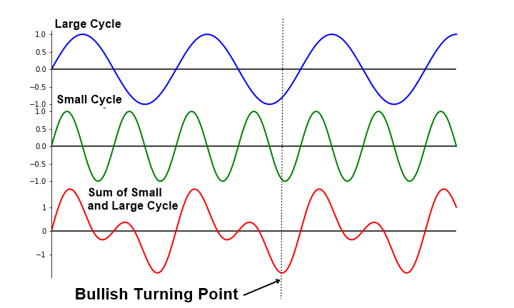
Figure 4.2-2: Conceptual drawing of global bullish turning point in small and large waves with deterministic cycles
We can only tell if current amplitude and wavelength could become a turning point with some measured certainty or uncertainty. However, we can never be sure for 100%. If each cycle only provides the probability to become peak or trough, then how can we estimate the confluence between small and large cycle of stochastic cycles? Probably, one way to do is calculating the joint probability between small and large cycles.
Figure 4.2-3: Uncertainty in the turning point prediction
To visualize this joint probability concept in our trading, consider we have one small cycle and one big cycle. Say that three fractal triangles in the small cycle are the child waves of one fractal triangle in the big cycle. In such case, we can calculate two turning point probability, one for child wave (Triangle 0), and the other one for mother wave (Triangle M0). Firstly, we can calculate the turning point probability for the Triangle 0, the child wave, based on its amplitude and wavelength (Figure 4.2-4).
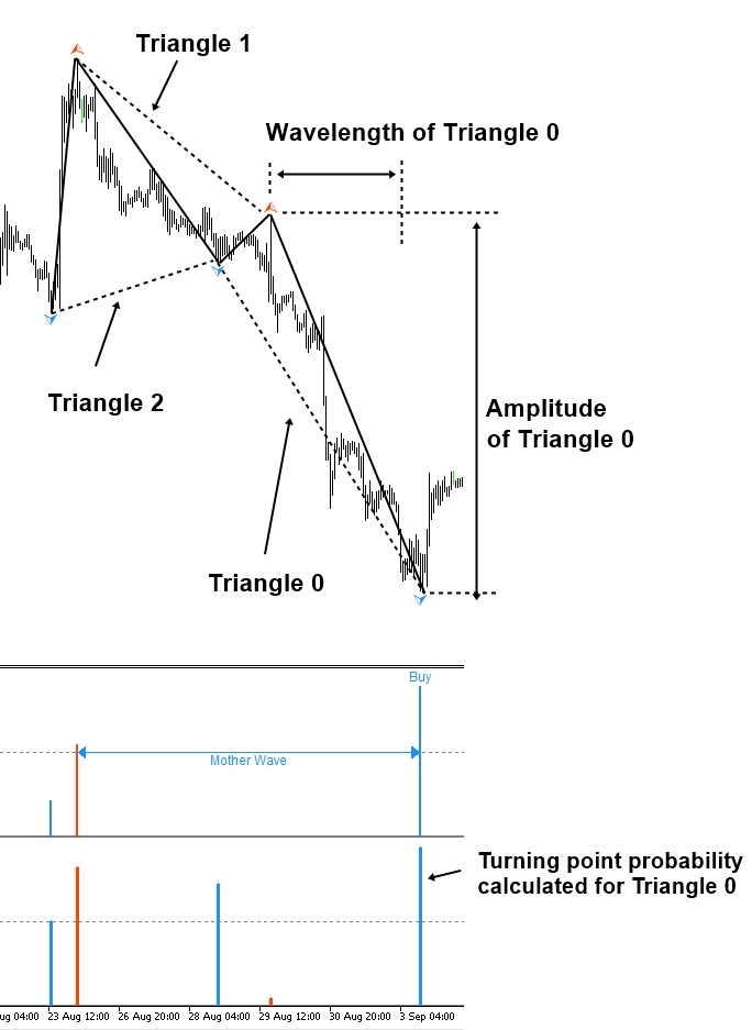
Figure 4.2-4: Calculating the turning point probability for small cycle (i.e. Triangle 0)
Next, we can calculate the turning point probability based on the amplitude and wavelength of Triangle M0, mother wave, in the big cycle (Figure 4.2-5). Then we use these two probabilities for Triangle 0 and Triangle M0 to calculate the joint probability. In fact, the most convenient form to represent the joint probability between two cycles is using the matrix representation like the correlation matrix.
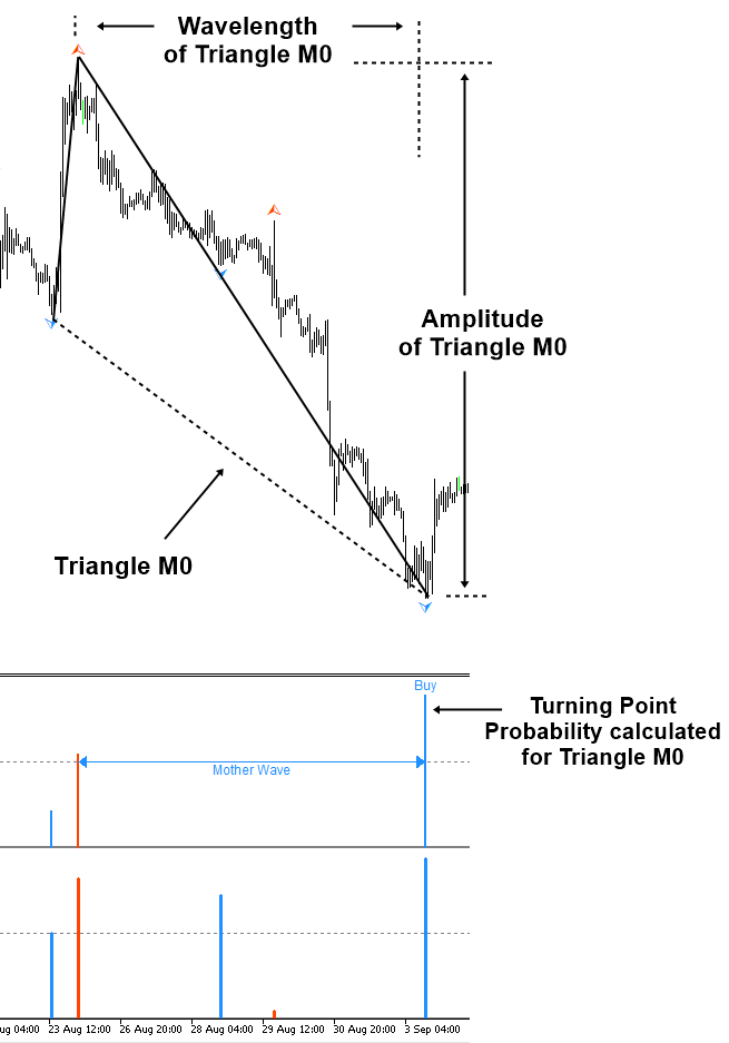
Figure 4.2-5: Calculating the turning point probability for large cycle (i.e. Triangle M0)
If we name the small cycle as Cycle 0 and if we name the big cycle as Cycle 1, then we can put all the probabilities including the joint probability and probability for each cycle in one table (Figure 4.2-6). As in the correlation matrix, the diagonal probability indicates the self-probability of each cycle. The top right probability indicates the joint probability between small cycle (i.e. Cycle 0) and big cycle (i.e. Cycle 1). Probabilities below the diagonal probabilities are the mirror of the probabilities above the diagonal probabilities.
In terms of our trading, we have two joint probability matrix. One matrix is for the calculated probabilities in price dimension using the amplitude of Triangle 0 and Triangle M0. The other matrix is for the calculated probabilities in time dimension using the wavelength of Triangle 0 and Triangle M0. For our trading, we have to watch out when there is higher joint probability either in price or in time. Higher joint probability is equivalent to the global turning point we have shown in the case of deterministic cycle. In our example, we have the joint probability between Triangle 0 and Triangle M0 is 88.9% in price dimension. It is 86.7% in time dimension. In this case, the joint probability is high enough to alert you for the turning point in the market.
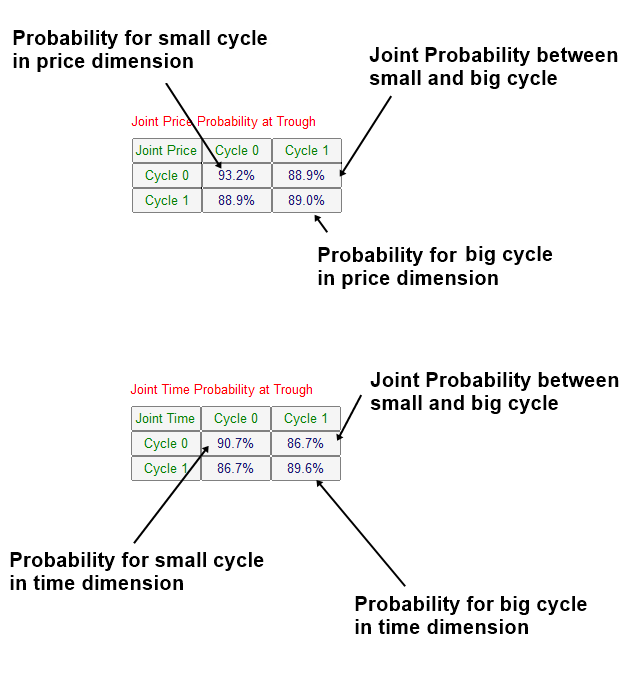
Figure 4.2-6: Joint Probability Matrix for small cycle (i.e. Cycle 0) and large cycle (i.e. Cycle 1)
You might find this matrix table overkill for the case of two cycles. However, when we have to calculate the joint probability for more than three cycles, then you would really appreciate this matrix representation. It is always better to stick with convention rather than creating our own method. If you get used to the joint probability matrix with two cycles, it is easy to understand the joint probability matrix with three or more cycles (Figure 4.2-7 and Figure 4.2-8).
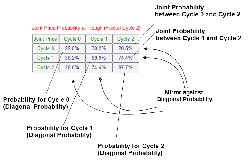
Figure 4.2-7: Joint Probability Matrix for small cycle (i.e. Cycle 0), middle cycle (i.e. Cycle 1), and large cycle (i.e. Cycle 2) in price dimension
When we inspect the joint probability matrix, we can put equal weight on price and time. Especially, we need to take bigger caution if the probability or joint probability in the higher cycle is big. For example, we have reasonably big joint probability between Cycle 1 and Cycle 2 in price dimension. At the same time, we can observe even bigger joint probability between Cycle 1 and Cycle 2 in time dimension. Since we have high probability in Cycle 1 and Cycle 2, we can care less on the probability in Cycle 0, the small cycle.
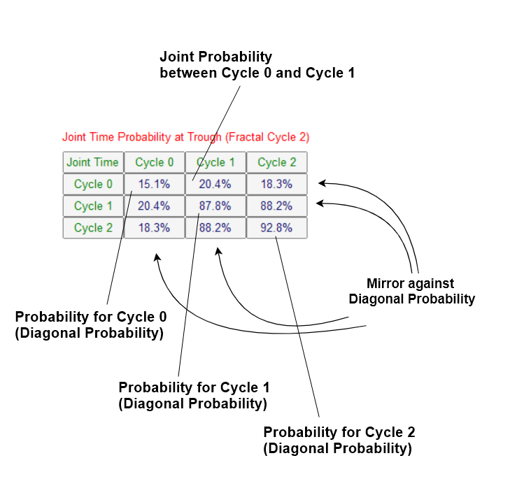
Figure 4.2-8: Joint Probability Matrix for small cycle, middle cycle, and large cycle in time dimension
High joint probability in time dimension tells us that bearish market was continued for prolonged period (Figure 4.2-9). At the same time, price moved deep enough for possible turning point. If there is any fundamental and political reason for bullish market, then this could be good opportunity to ride a big bullish market.
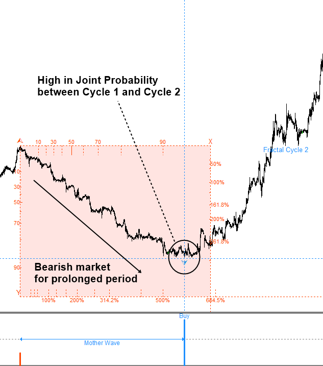
Figure 4.2-9: Predicting global turning point with high joint probability in price and time
Now we have covered how to read the joint probability matrix and how to use them in our trading. There are few more points you need to understand about the joint probability.
Firstly, the Joint Probability can be only calculated when the peak of small cycle is overlapping with the peak of large cycle. Likewise, it can be only calculated if the trough of small cycle is overlapping with the trough of large cycle.
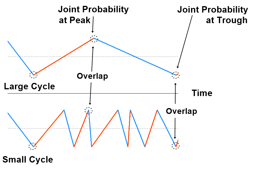
Figure 4.2-10: Demonstration of overlapping peak and trough in small and large cycles
Secondly, calculating joint probability always requires the probability of each cycle and you need at least two of them. In another words, if we cannot calculate probability for each cycle, then we do not have joint probability either. Also having only one probability does not help to calculate the joint probability either.
Finally, the joint probability helps to make the statistical prediction on the chance of two events to happen together. In our case, the Joint Probability describes the chance that one fractal triangle will end and new fractal triangle will start in both small and large cycles. This is the equivalent concept in the stochastic cycle to the global turning point in the deterministic cycle. Hence, this often provides you the most robust entry at which current trend changes its direction. However, this does not mean that you have to wait for the sufficiently high joint probability in your trading always. When the joint probability is not noticeable, you can use the probability for each cycle too. In this case, just stick to the Geometric prediction equation. In another words, you need to find the geometric regularity to justify your statistical regularity, which is the turning point probability in this case. It is even better if you do have some knowledge on the surrounding market condition.
Geometric Prediction (General version) = statistical regularity + geometric regularity + surrounding knowledge around object
Some More Tips about Mother Wave and Child Wave with Joint Probability
The “Mother Wave” and “Child Wave” concept is a trading strategy in forex trading that focuses on identifying trends and potential reversal points in the market. This strategy is based on the Elliott Wave Theory, which suggests that market movements unfold in repetitive patterns or waves. The “Mother Wave” represents the larger trend, while the “Child Wave” represents a smaller correction within that trend. Here’s how the concept works:
Mother Wave:
- Definition: The Mother Wave refers to the larger, primary trend in the market. It consists of the main directional movement that traders aim to identify and ride for profits. The Mother Wave can be bullish or bearish, depending on whether the overall market sentiment is bullish or bearish.
- Characteristics: The Mother Wave typically consists of multiple Elliott Wave impulse waves in the direction of the primary trend. These waves represent the strong, sustained movements that drive the market in the direction of the prevailing trend.
Child Wave:
- Definition: The Child Wave, also known as a corrective wave, is a smaller counter-trend movement within the larger trend represented by the Mother Wave. It is a temporary interruption or correction against the primary trend.
- Characteristics: The Child Wave often appears as a smaller-scale correction within the larger trend, typically taking the form of Elliott Wave corrective patterns such as zigzags, flats, or triangles. It tends to be shorter in duration and magnitude compared to the primary trend represented by the Mother Wave.
Joint Probability:
- Definition: Joint probability refers to the likelihood of two or more events occurring together. In the context of the Mother Wave and Child Wave strategy, joint probability involves assessing the likelihood of both waves aligning and signaling potential trading opportunities.
- Application: Traders using the Mother Wave and Child Wave strategy look for alignment between the larger trend represented by the Mother Wave and the smaller corrections represented by the Child Wave. By analyzing the joint probability of these waves, traders aim to identify potential entry and exit points in the market.
- Confirmation: Confirmation of alignment between the Mother Wave and Child Wave may come from additional technical indicators, such as momentum oscillators, trendlines, or Fibonacci retracement levels. Traders seek confirmation signals that validate the joint probability of both waves and support their trading decisions.
The Mother Wave and Child Wave concept in forex trading emphasizes the importance of understanding the interplay between larger trends and smaller corrections within the market. By assessing the joint probability of these waves and looking for confirmation signals, traders aim to make more informed trading decisions and capitalize on profitable opportunities. As with any trading strategy, thorough backtesting and practice are essential to validate the effectiveness of the approach.
About this Article
This article is the part taken from the draft version of the Book: Predicting Forex and Stock Market with Fractal Pattern. This article is only draft and it will be not updated to the completed version on the release of the book. However, this article will serve you to gather the important knowledge in financial trading. This article is also recommended to read before using Fractal Pattern Scanner, which is available for MetaTrader or Optimum Chart.
Below is the landing page for Fractal Pattern Scanner for MetaTrader 4 and MetaTrader 5. The same products are available on www.mql5.com too.
https://www.mql5.com/en/market/product/49170
https://www.mql5.com/en/market/product/49169
https://algotrading-investment.com/portfolio-item/fractal-pattern-scanner/
Below is the landing page for Optimum Chart
https://algotrading-investment.com/2019/07/23/optimum-chart/
Related Products